Cost function, back propagation, forward propagation, unrolling parameters, gradient checking, and random initialization.
1. Cost Function and Back Propagation
I would like to give full credits to the respective authors as these are my personal python notebooks taken from deep learning courses from Andrew Ng, Data School and Udemy :) This is a simple python notebook hosted generously through Github Pages that is on my main personal notes repository on https://github.com/ritchieng/ritchieng.github.io. They are meant for my personal review but I have open-source my repository of personal notes as a lot of people found it useful.
1a. Cost Function
- Neural Network Introduction
- One of the most powerful learning algorithms
- Learning algorithm for fitting the derived parameters given a training set
- Neural Network Classification
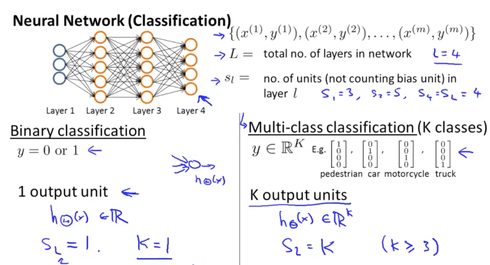
- Cost Function for Neural Network
- Two parts in the NN’s cost function
- First half (-1 / m part)
- For each training data (1 to m)
- Sum each position in the output vector (1 to K)
- For each training data (1 to m)
- Second half (lambda / 2m part)
- Weight decay term
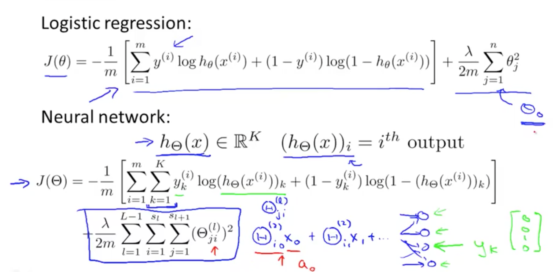
- Weight decay term
- First half (-1 / m part)
- Two parts in the NN’s cost function
1b. Overview
- Forward propagation
- Algorithm that takes your neural network and the initial input (x) and pushes the input through the network
- Back propagation
- Takes output from your neural network H(Ɵ)
- Compares it to actual output y
- Calculates H(Ɵ)’s deviation from actual output
- Takes the error H(Ɵ) - y from layer L
- Back calculates error associated with each unit from the preceding layer L - 1
- Error calculated from each unit used to calculate partial derivatives
- Use partial derivatives with gradient descent to minimise cost function J(Ɵ)
- Takes output from your neural network H(Ɵ)
- Basic things to note
- Ɵ matrix for each layer in the network
- This has each node in layer l as one dimension and each node in l+1 as the other dimension
- Δ matrix for each layer
- This has each node as one dimension and each training data example as the other
- Ɵ matrix for each layer in the network
1c. Backpropagation Algorithm
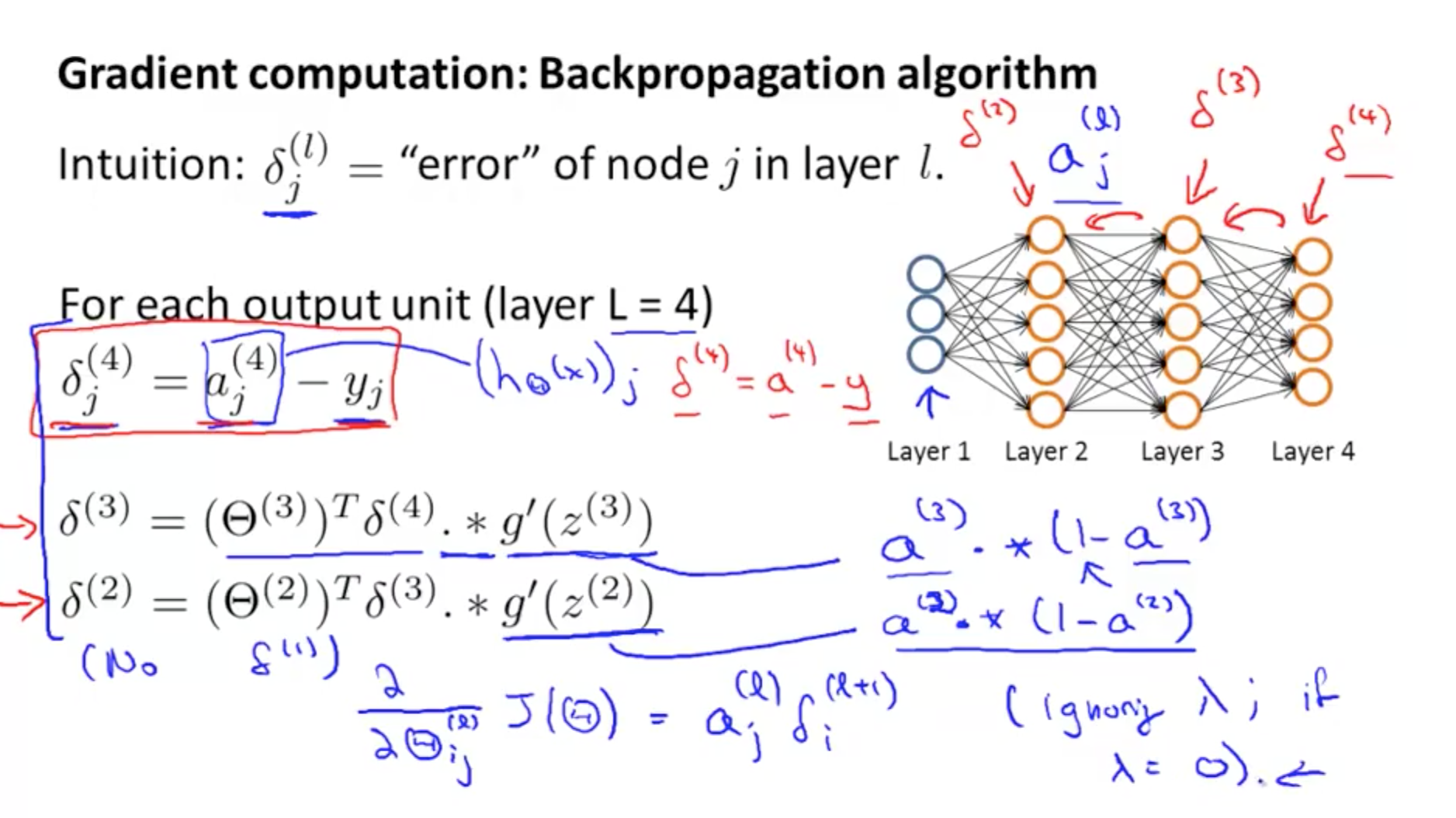
- Gradient Computation
- Purpose is to find parameters Ɵ that minimizes J(Ɵ)
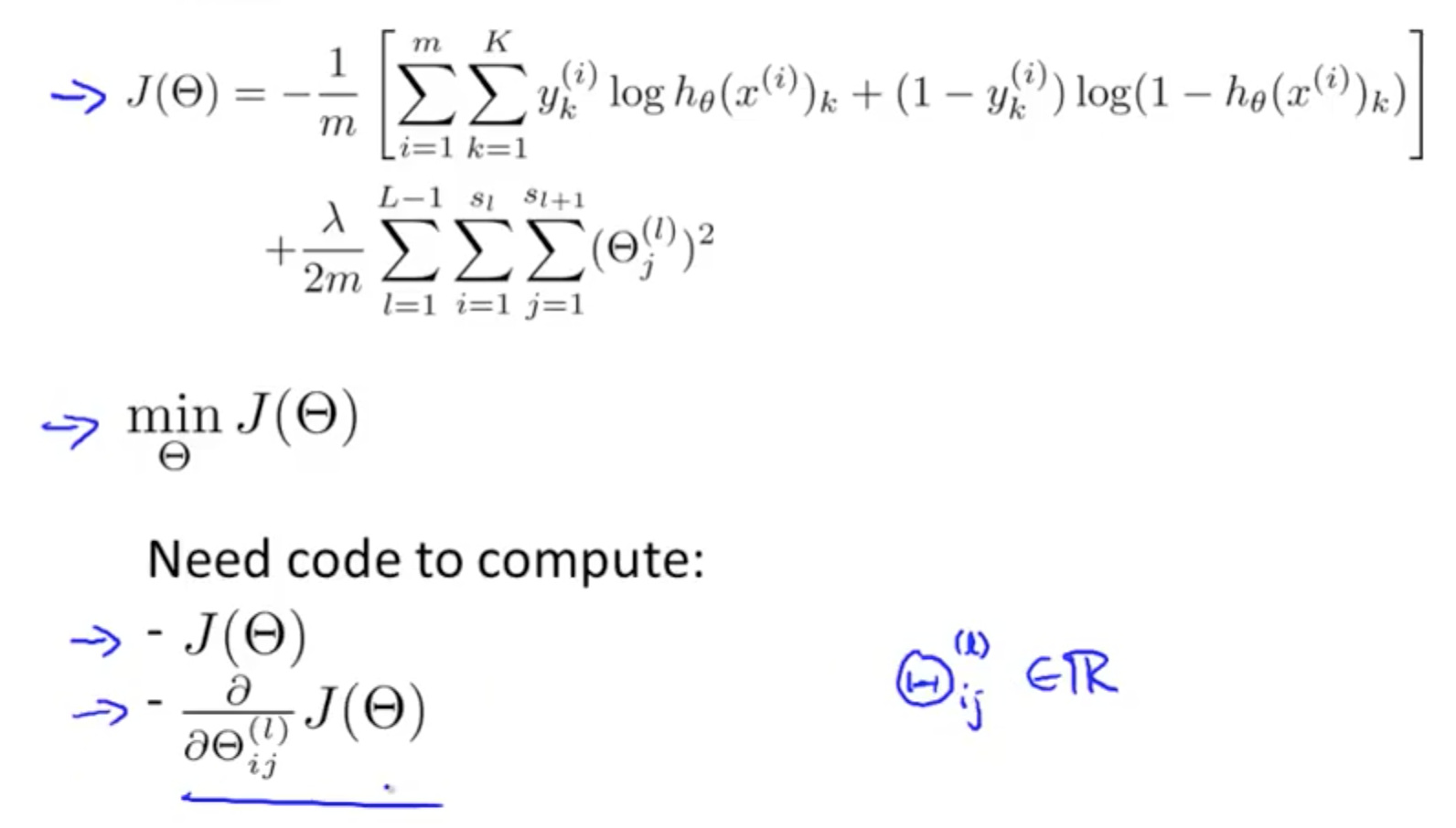
- Purpose is to find parameters Ɵ that minimizes J(Ɵ)
- Forward Propagation
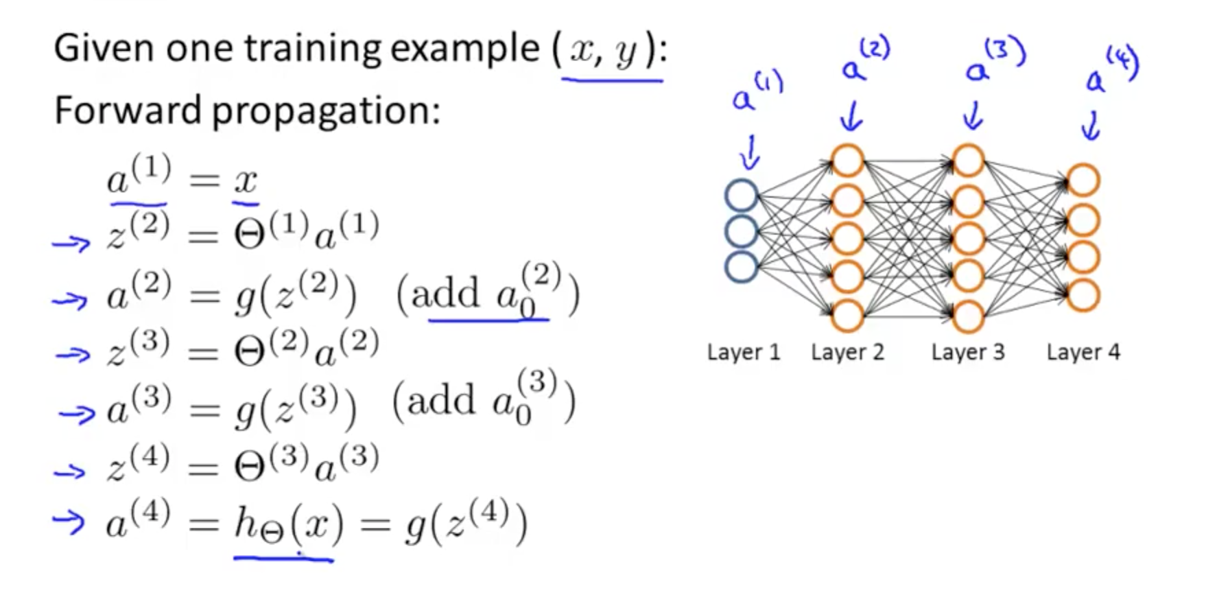
- Backpropagation Equation
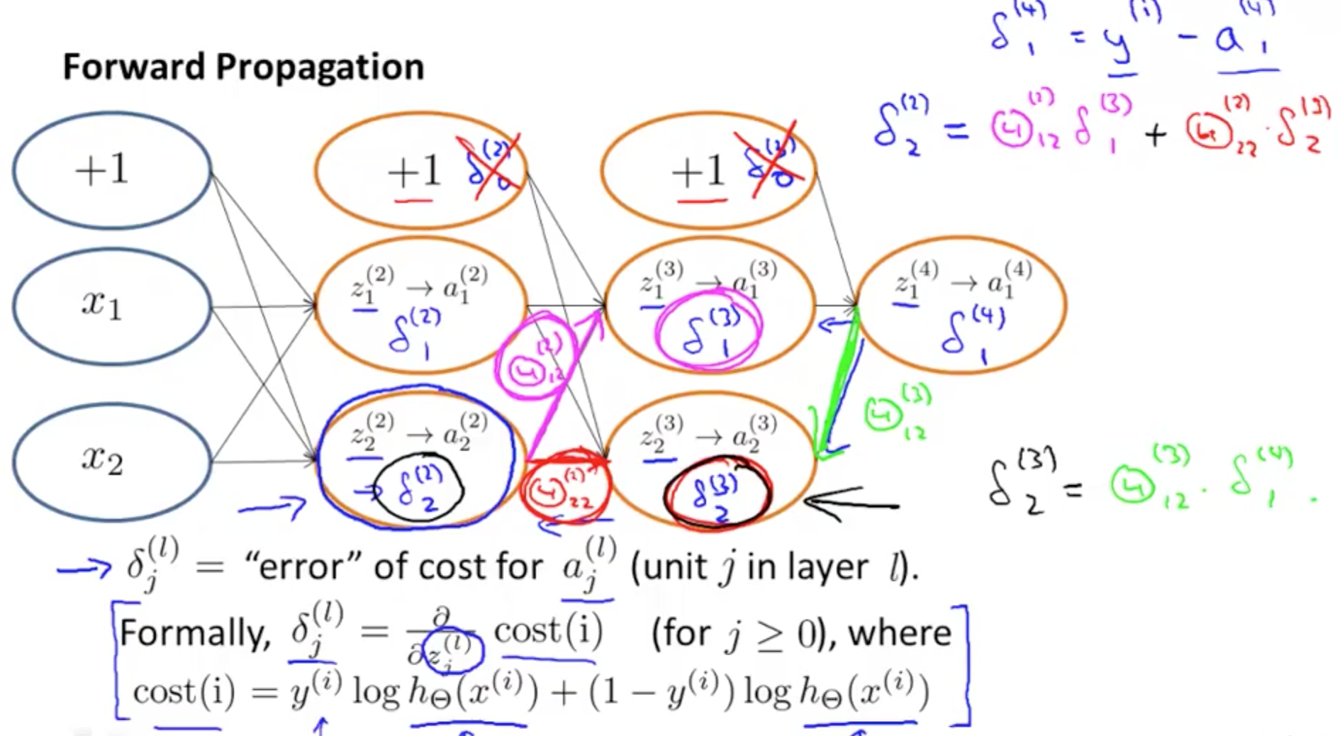
- For each node we can calculate δj^l
- This is the error of node j in layer l
- aj^l is the activation of node j in layer l
- activation would have some error compared to the “real” value
- delta calculates this error
- But the “real” value is an issue
- The neural network is an artificial construct we made
- We have to use the actual output, y and work from there
- Work from the last/output layer, L
- If L = 4
- delta^4 = a^4 - y
- We can determine error in the preceding layers once we’ve the error from the output layer
- delta^3
- delta^2
- There is no error in the first layer as it’s simply the actual input x
- Once we get the deltas, we can calculate the gradient or the partial derivative of the cost function
- Terms in equation

- Dimensions

- For each node we can calculate δj^l
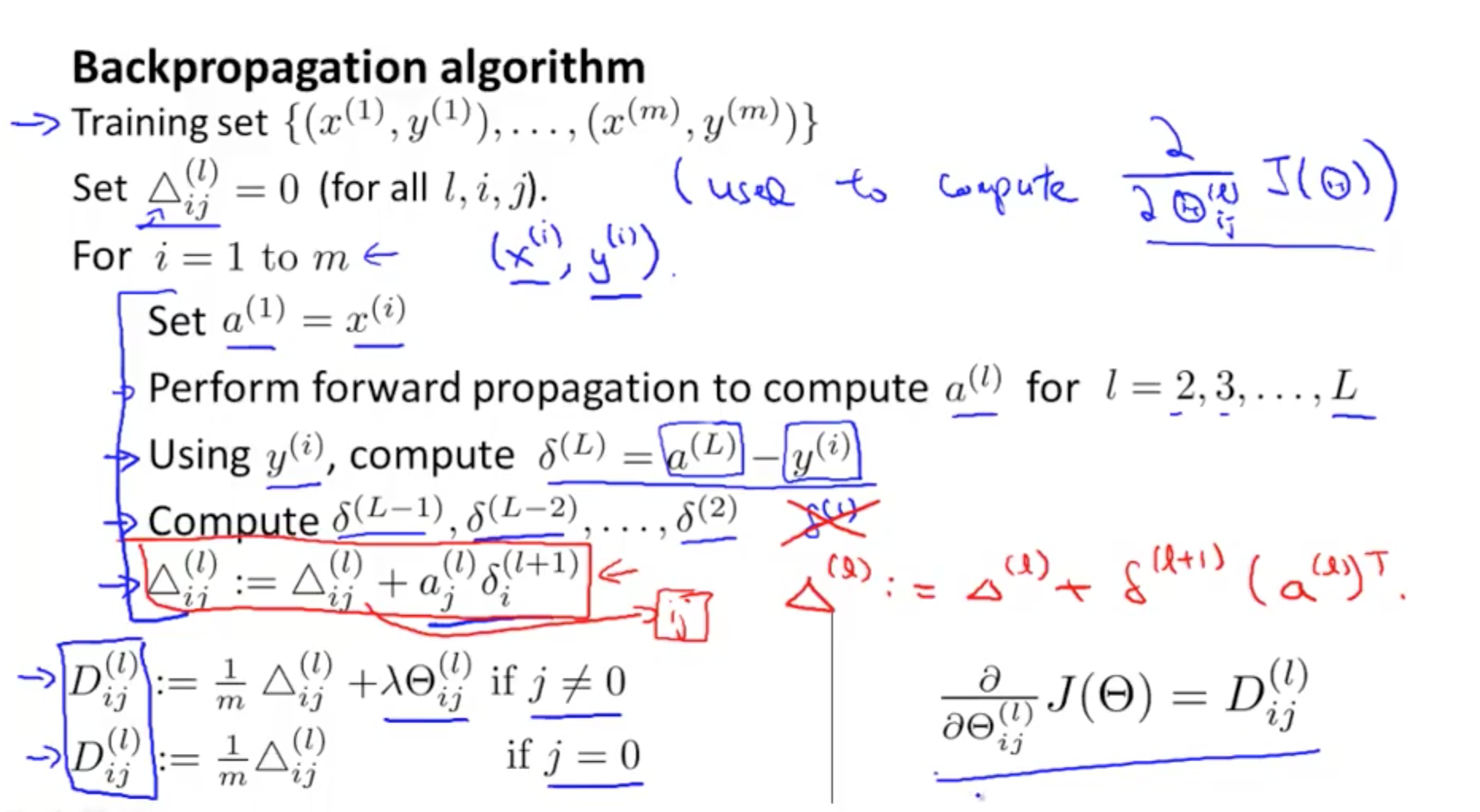
- Backpropagation Algorithm
1d. Backpropagation Intuition
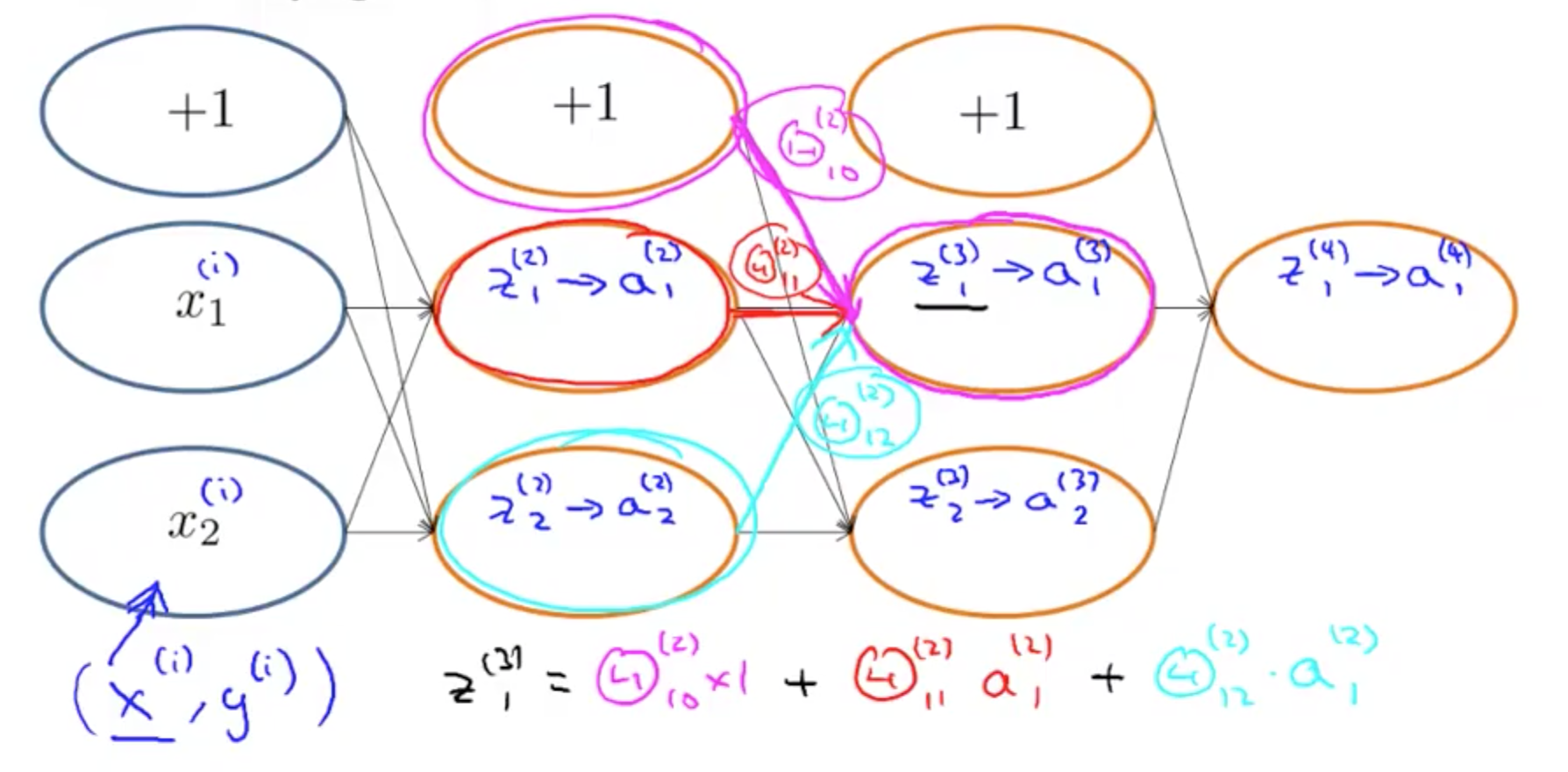
- Forward Propagation
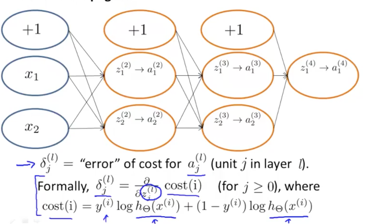
- Backpropagation’s cost function with 1 output unit

2. Backpropagation in Practice
2a. Unrolling Parameters
- Advanced optimization
- Issue here is that we’ve to unroll the matrices into vectors for the algorithm fminunc
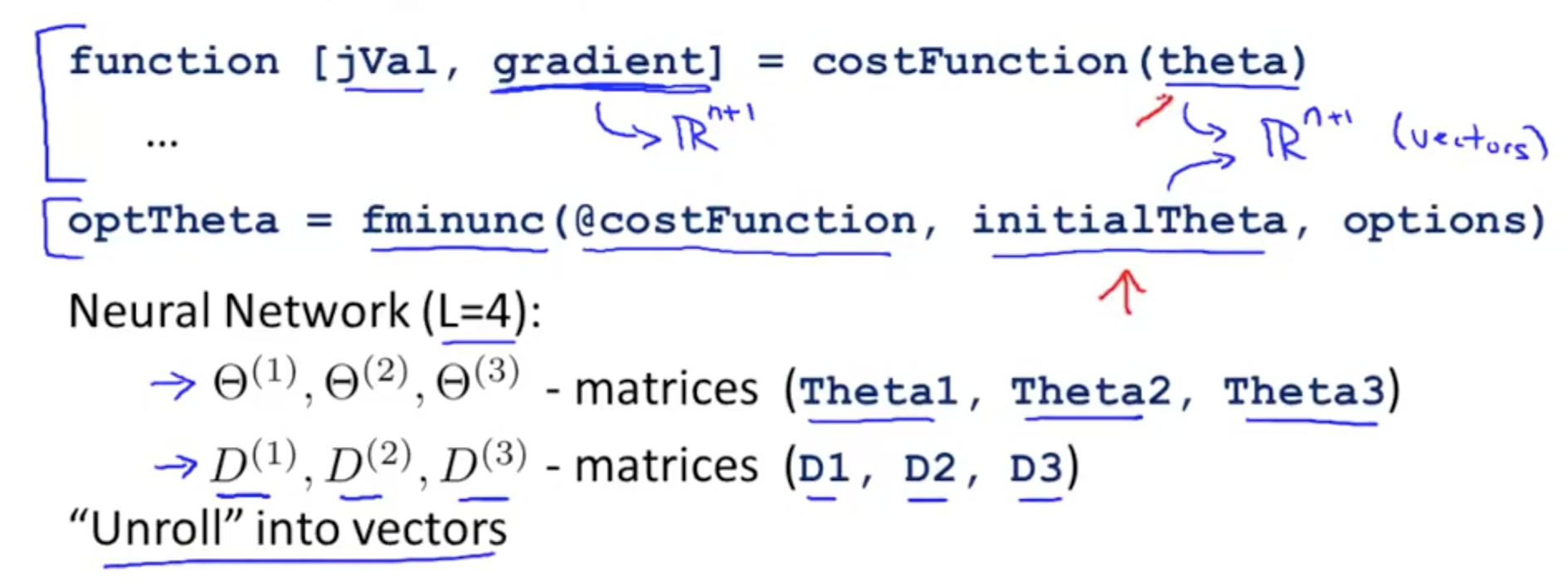
- Issue here is that we’ve to unroll the matrices into vectors for the algorithm fminunc
- Example
- s1 (layer 1 units) = 10
- s2 (layer 2 units) = 10
- s3 (layer 3 units) = 1
- Ɵ1(:) unrolls into a vector
- You can go back with reshape by pulling up each bunch of elements and reshape accordingly
- thetaVec(1:110) pulls up Ɵ1, the first 10 x 11 elements
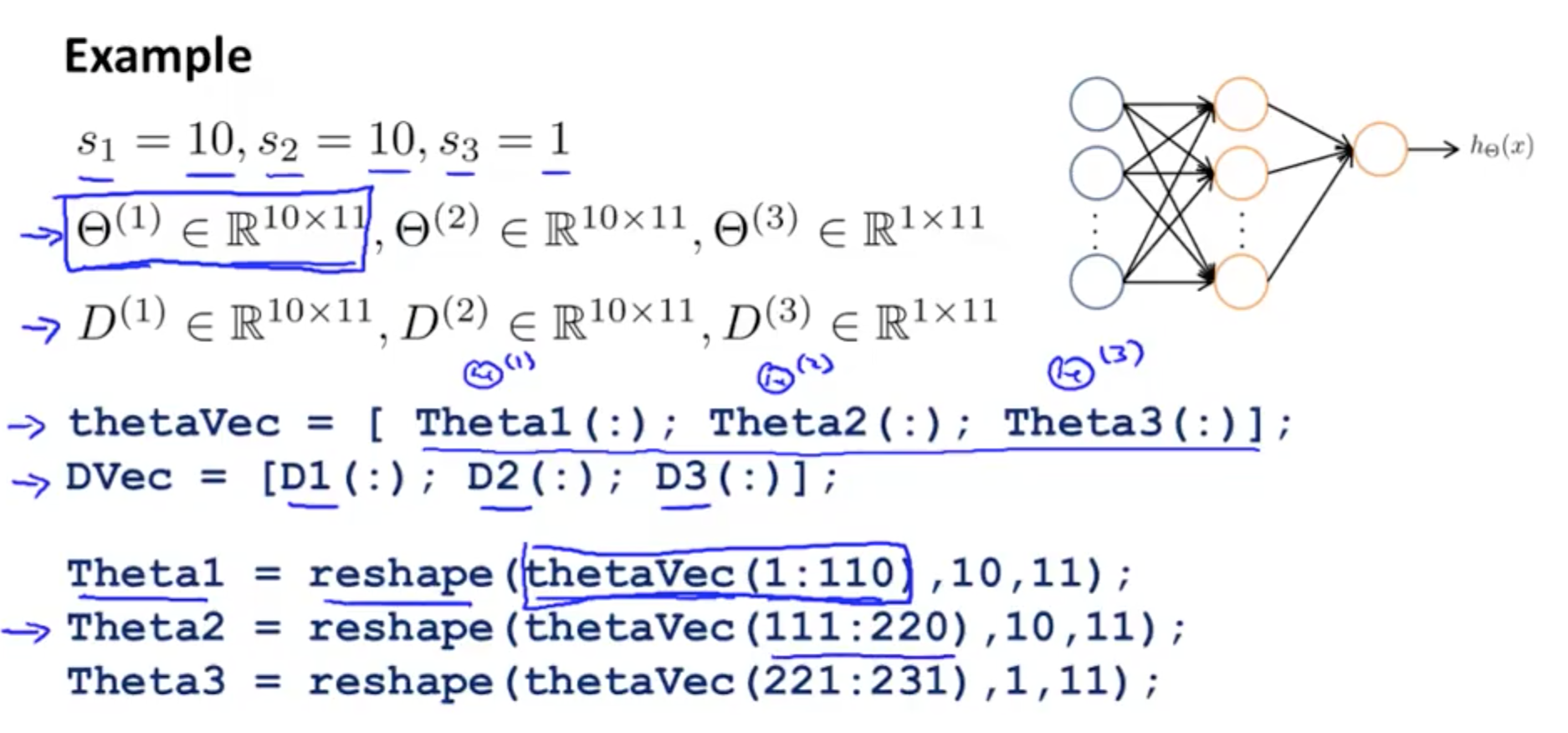
- thetaVec(1:110) pulls up Ɵ1, the first 10 x 11 elements
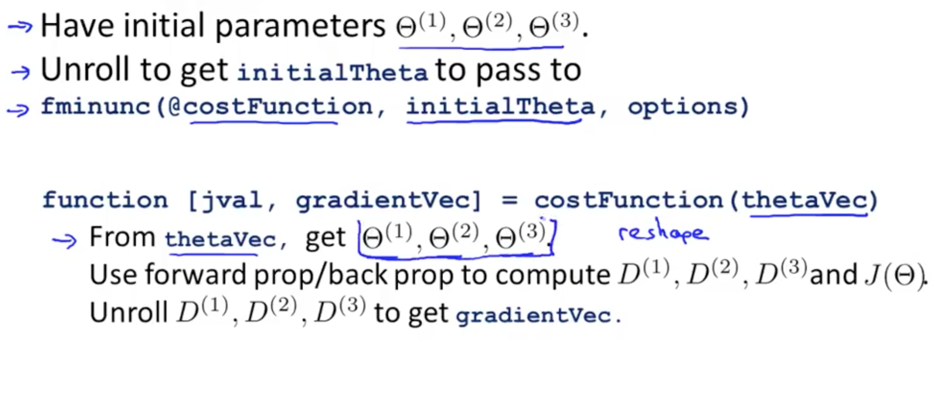
- Learning Algorithm
2b. Gradient Checking
- It might look like J(Ɵ) is decreasing
- But you might not know that there is a bug
- You can do gradient checking to ensure your implementation is 100% correct
- We can numerically estimate gradients
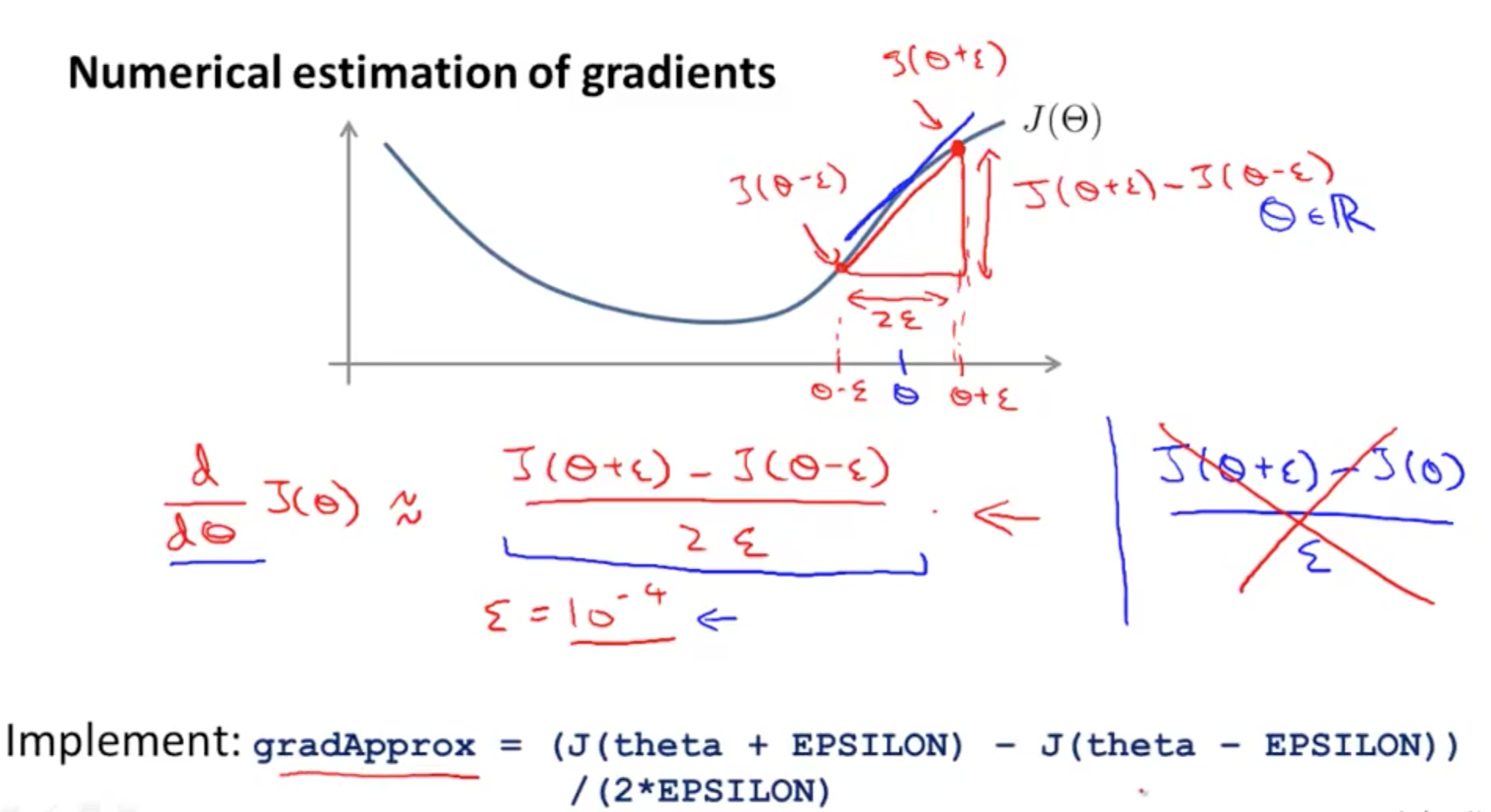
- Octave implementation
- n is the dimension of Ɵ
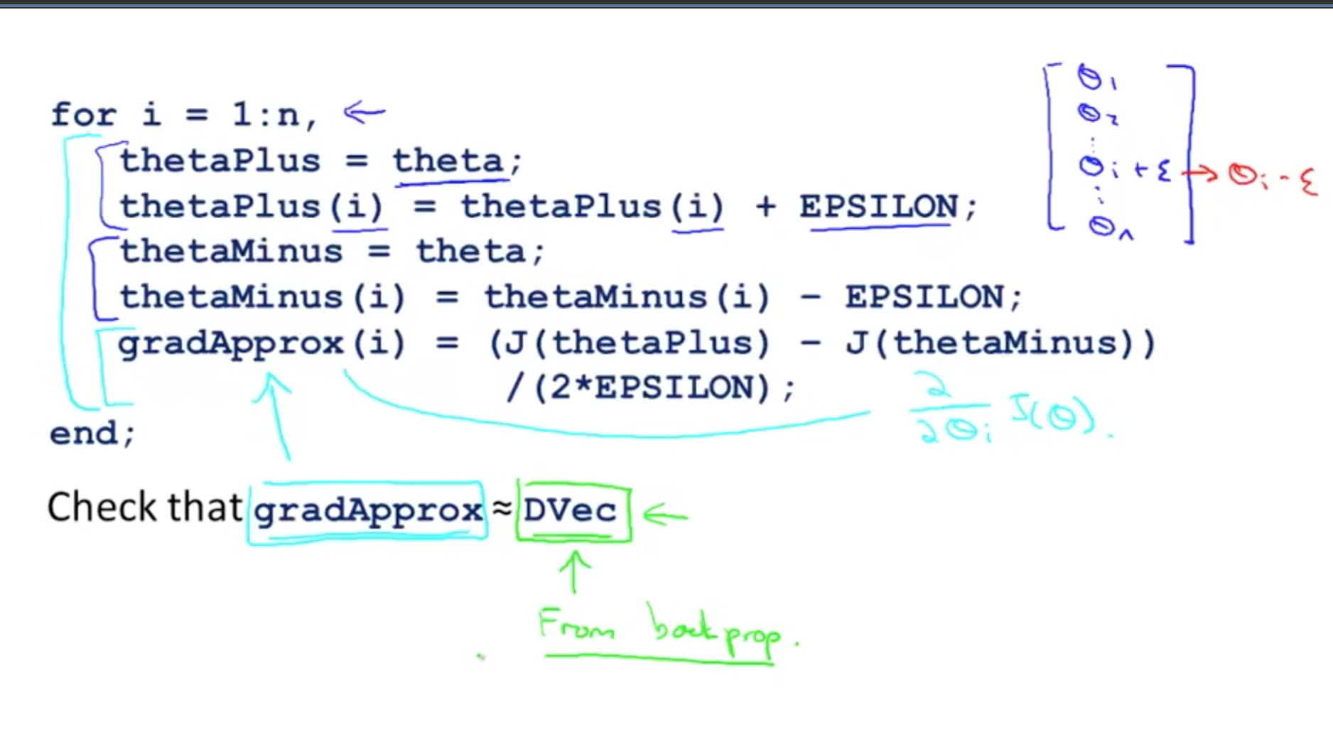
- n is the dimension of Ɵ
- Implementation Note
- Always turn off your numerical checking code as it’s very slow to execute
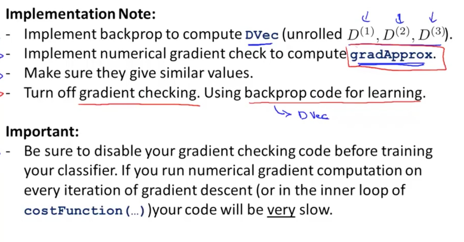
- Always turn off your numerical checking code as it’s very slow to execute
2c. Random Initialization
- Initial value of Ɵ
- Initialising Ɵ with zeros would not work for neural networks
- After each update, parameters corresponding to inputs going into each of two hidden units are identical
- You NN would not learn anything interesting
- Solution is to have a random initialisation
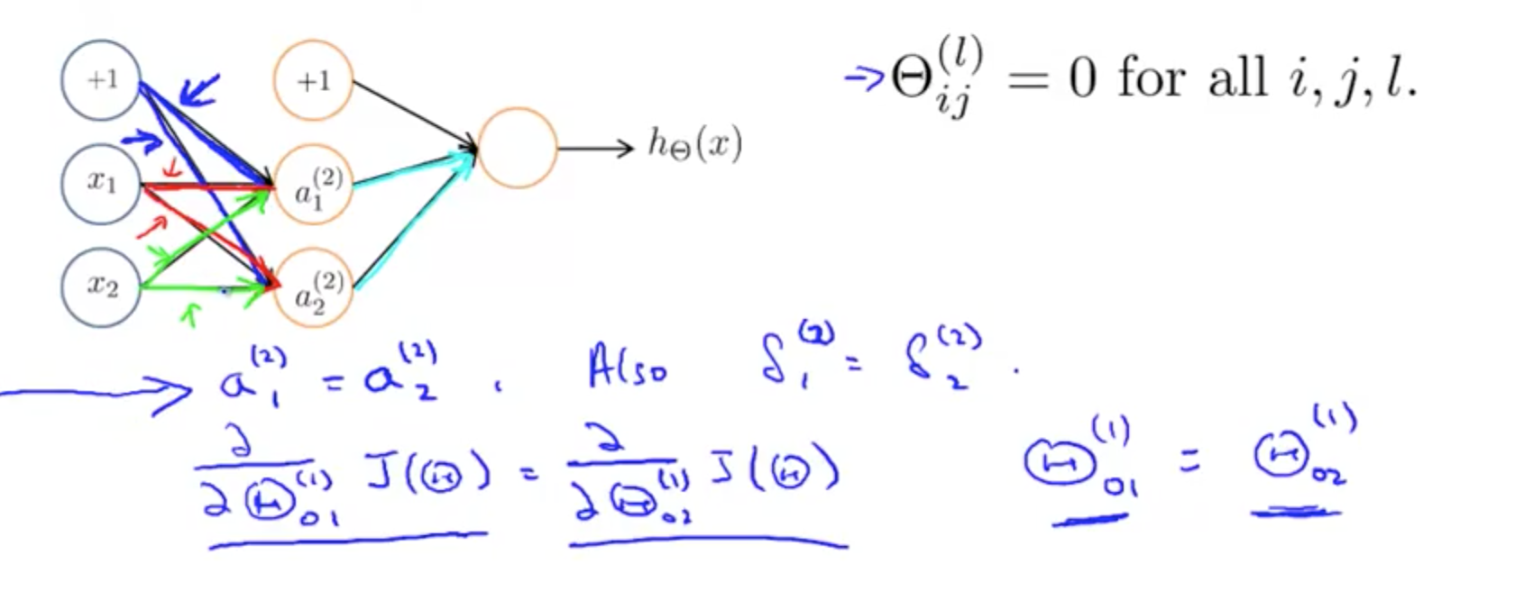
- Random initialization: symmetry breaking
- You will be able to use gradient descent or any advanced optimisation methods to find good values for theta
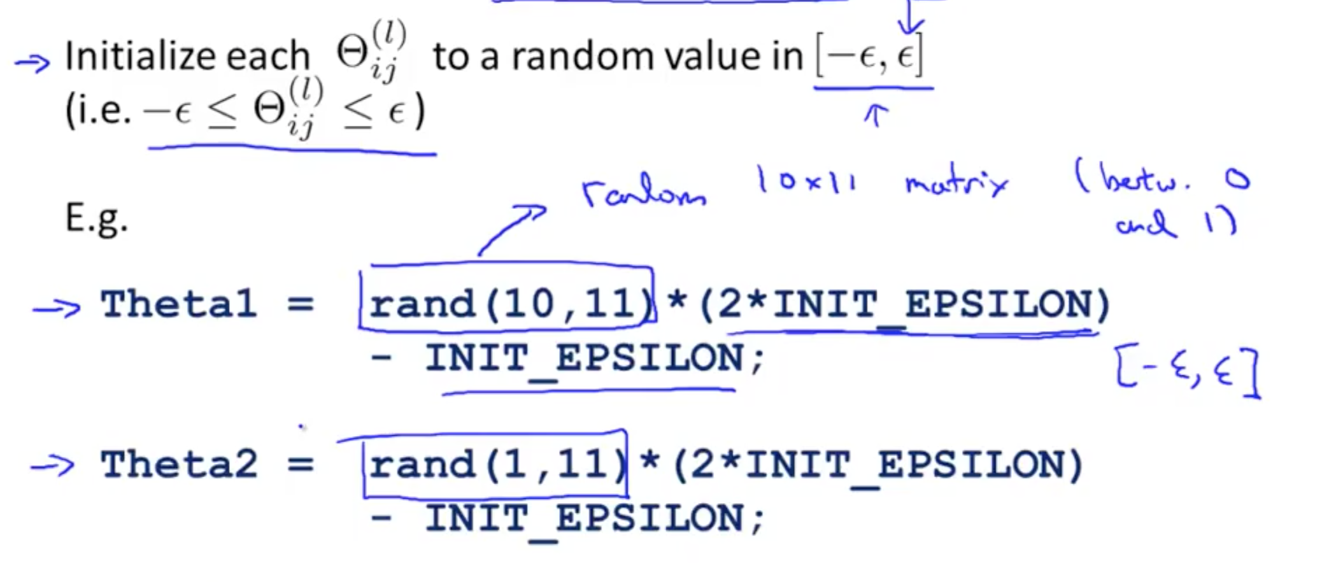
- You will be able to use gradient descent or any advanced optimisation methods to find good values for theta
2d. Putting everything together
- NN’s layers
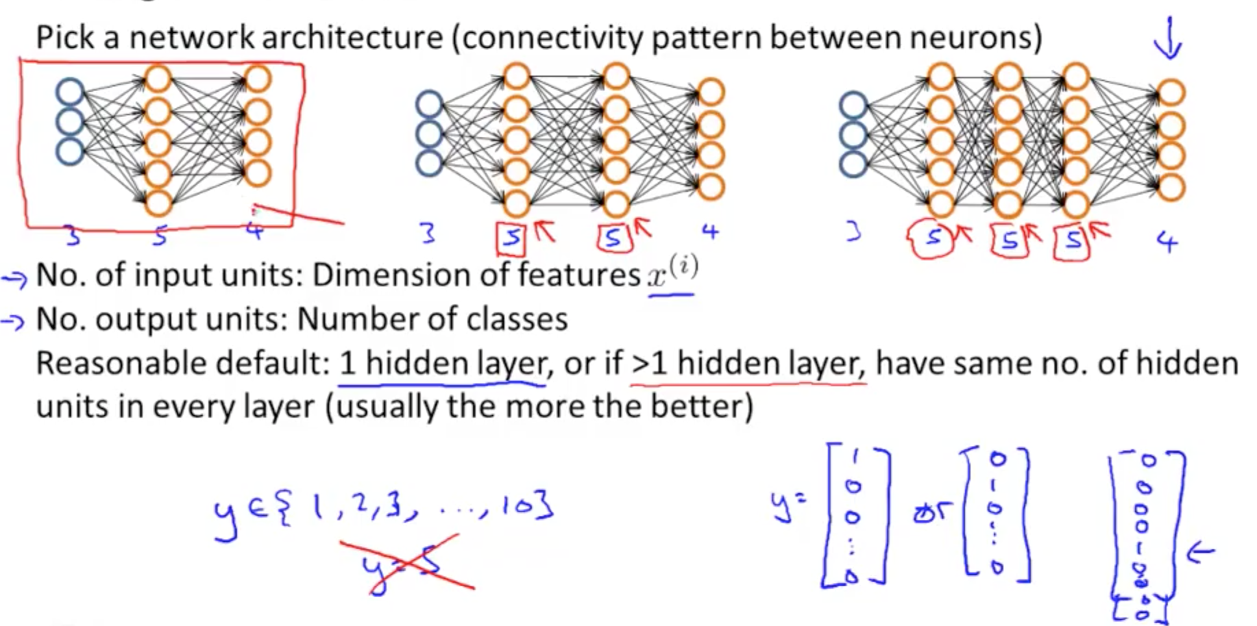
- Six steps for training a neural network
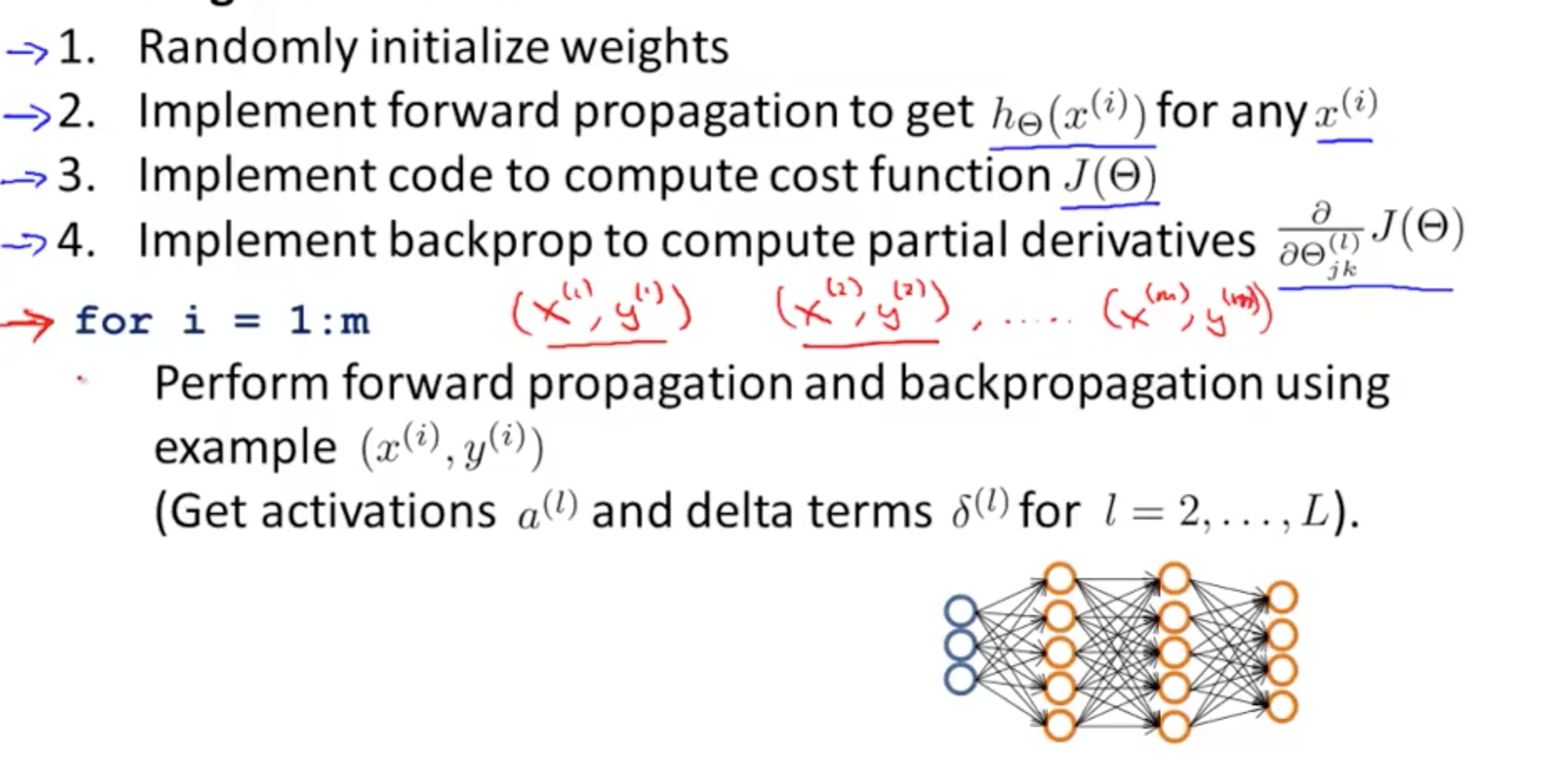
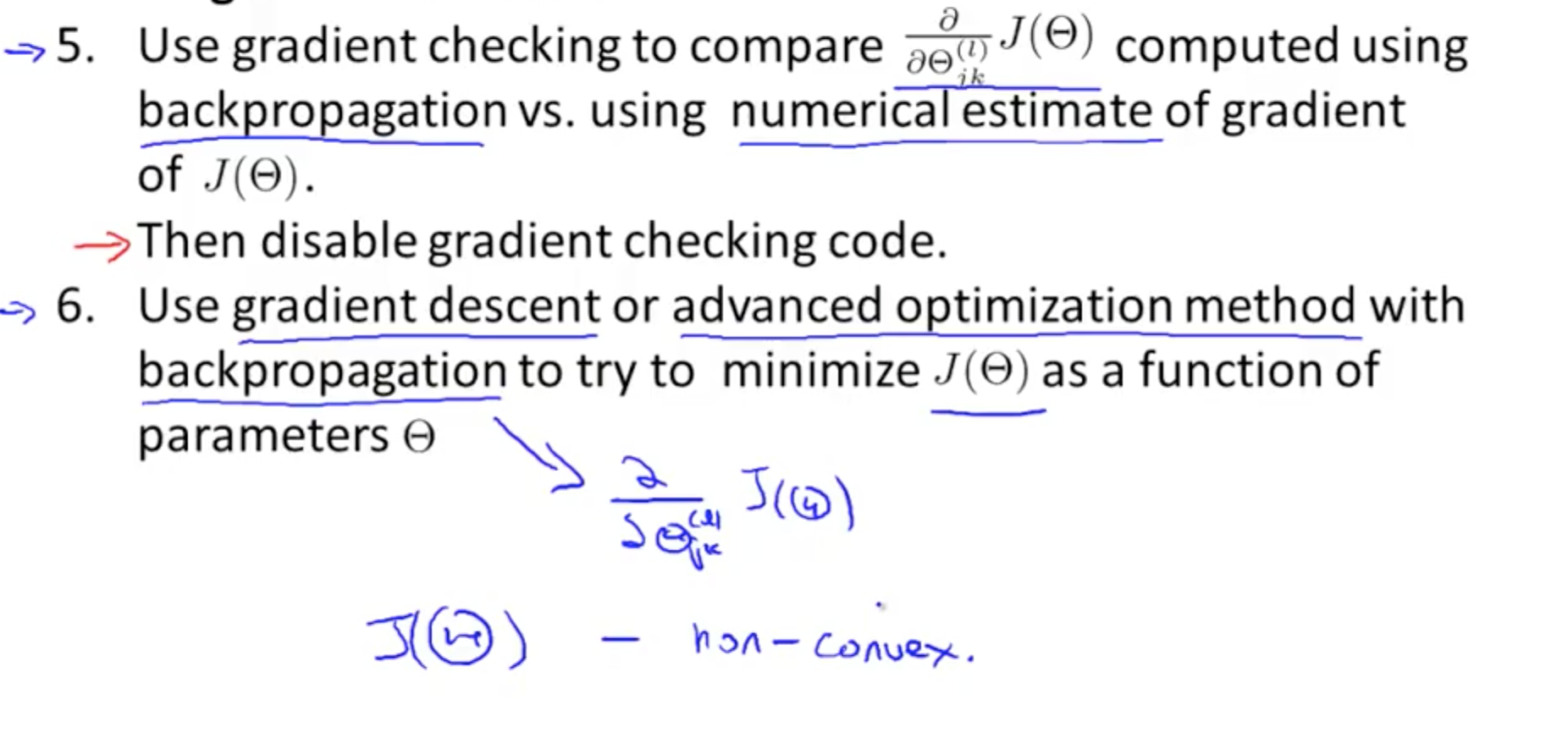
- J(Ɵ) closeness to actual values
- Gradient descent: taking little steps downhill to find lowest J(theta)
- Backpropagation: computing direction of gradient
- Able to fit non-linear functions
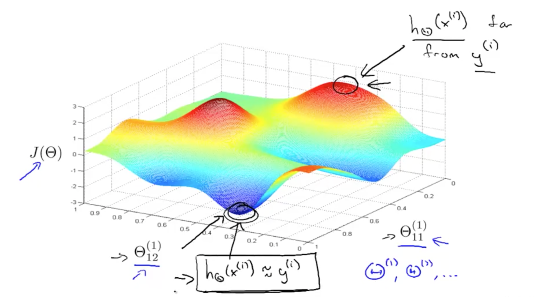
- Able to fit non-linear functions