Motivation of dimensionality reduction, Principal Component Analysis (PCA), and applying PCA.
1. Motivation
I would like to give full credits to the respective authors as these are my personal python notebooks taken from deep learning courses from Andrew Ng, Data School and Udemy :) This is a simple python notebook hosted generously through Github Pages that is on my main personal notes repository on https://github.com/ritchieng/ritchieng.github.io. They are meant for my personal review but I have open-source my repository of personal notes as a lot of people found it useful.
1a. Motivation I: Data Compression
- You are able to reduce the dimension of the data from 2D to 1D
- For example, pilot skill and pilot happiness can be reduced to pilot’s aptitude
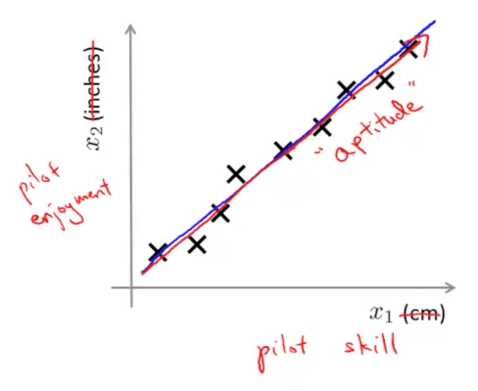
- Generally, you can reduce x1 and x2 to z1
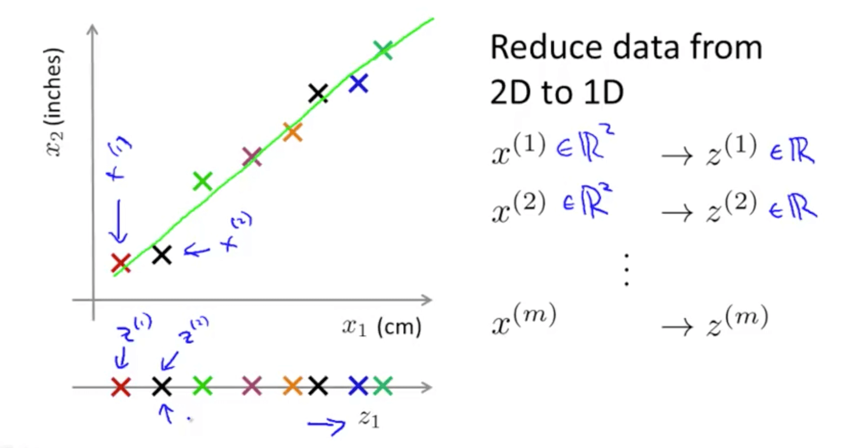
- For example, pilot skill and pilot happiness can be reduced to pilot’s aptitude
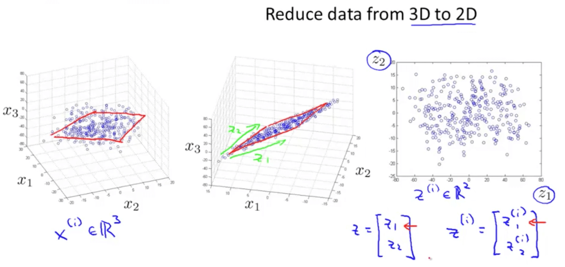
- Your are able to reduce the dimension of the data from 3D to 2D
- Project the data such that they lie on a plane
- Specify two axes
- z1
- z2
- You would then be able to reduce the data’s dimension from 3D to 2D
1b. Motivation II: Visualization
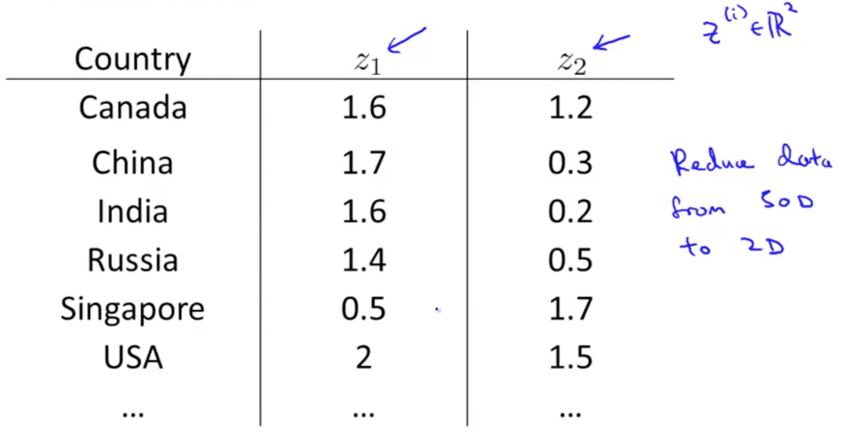
- Given a set of data, how are able to examine the data such as this?
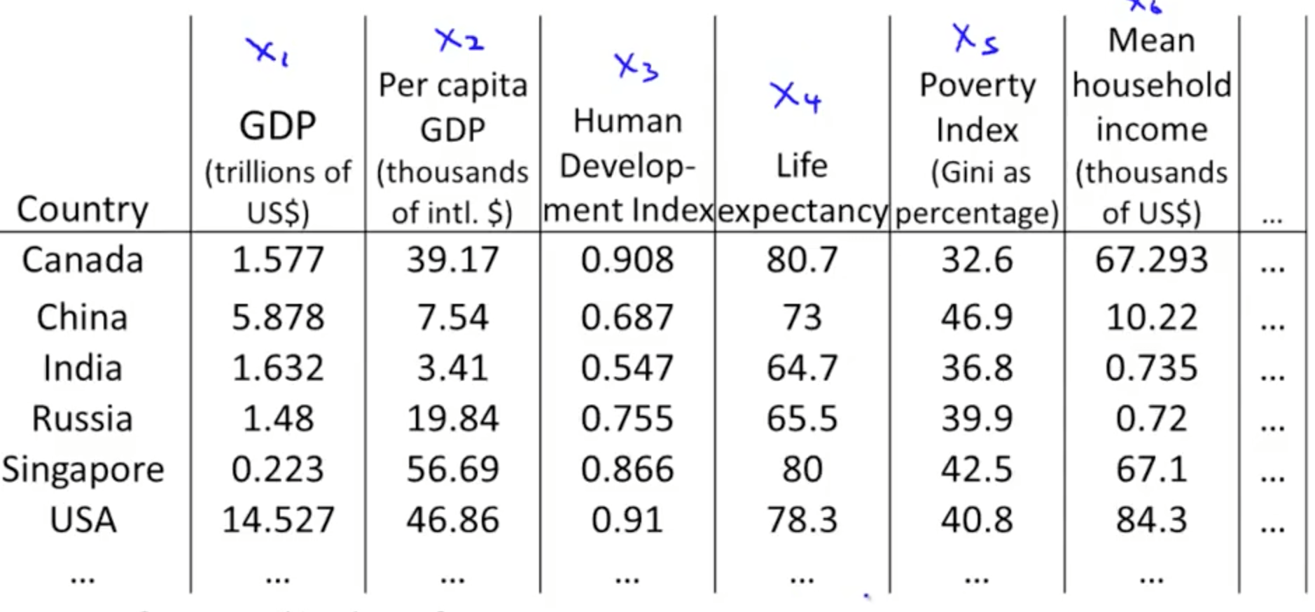
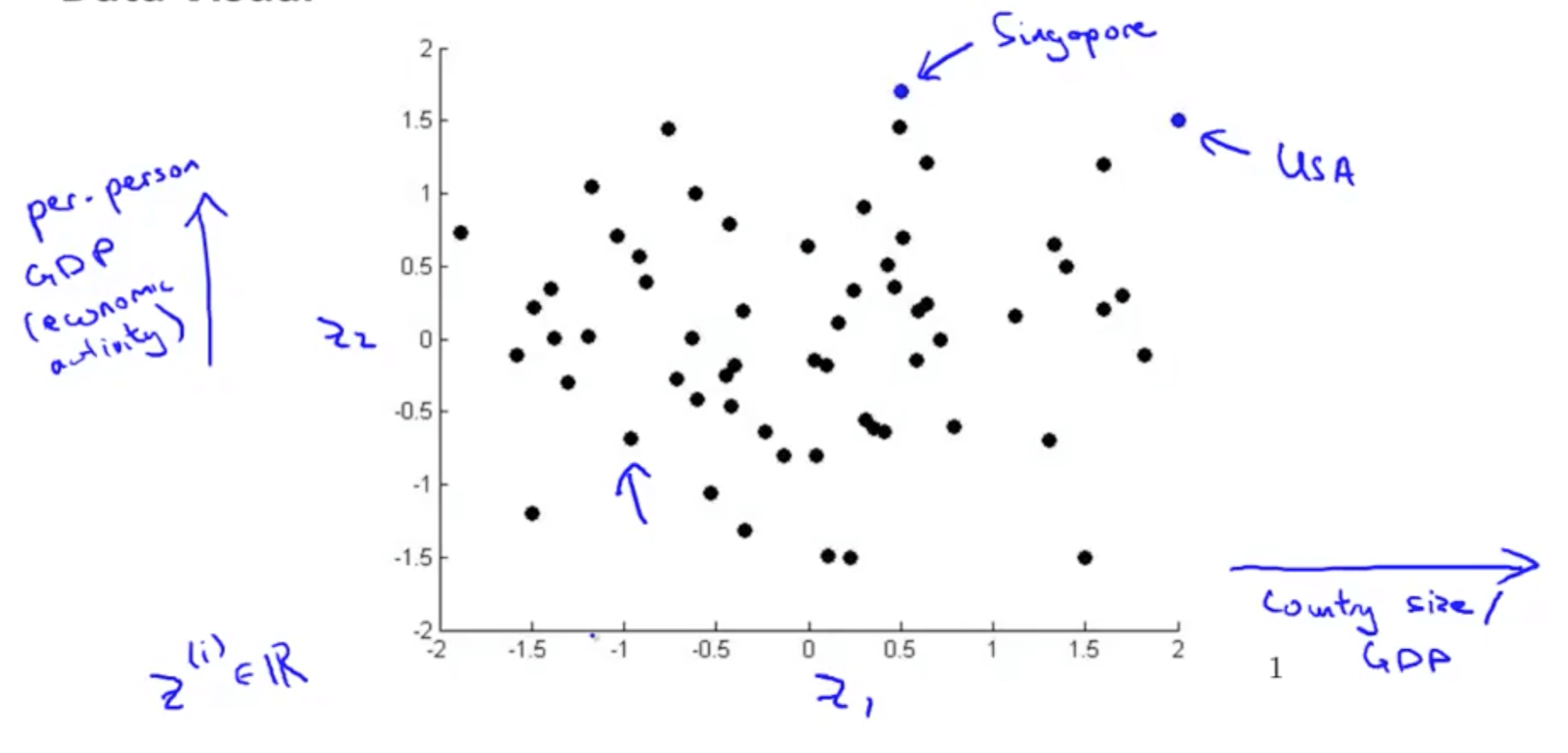
- We can use reduce the data’s dimensionality from 50D to 2D
- Typically we do not know what the 2 dimensions’ meanings are
- But we can make sense of out of the 2 dimensions
2. Principal Component Analysis (PCA)
2a. PCA Problem Formation
- Let’s say we have the following 2D data
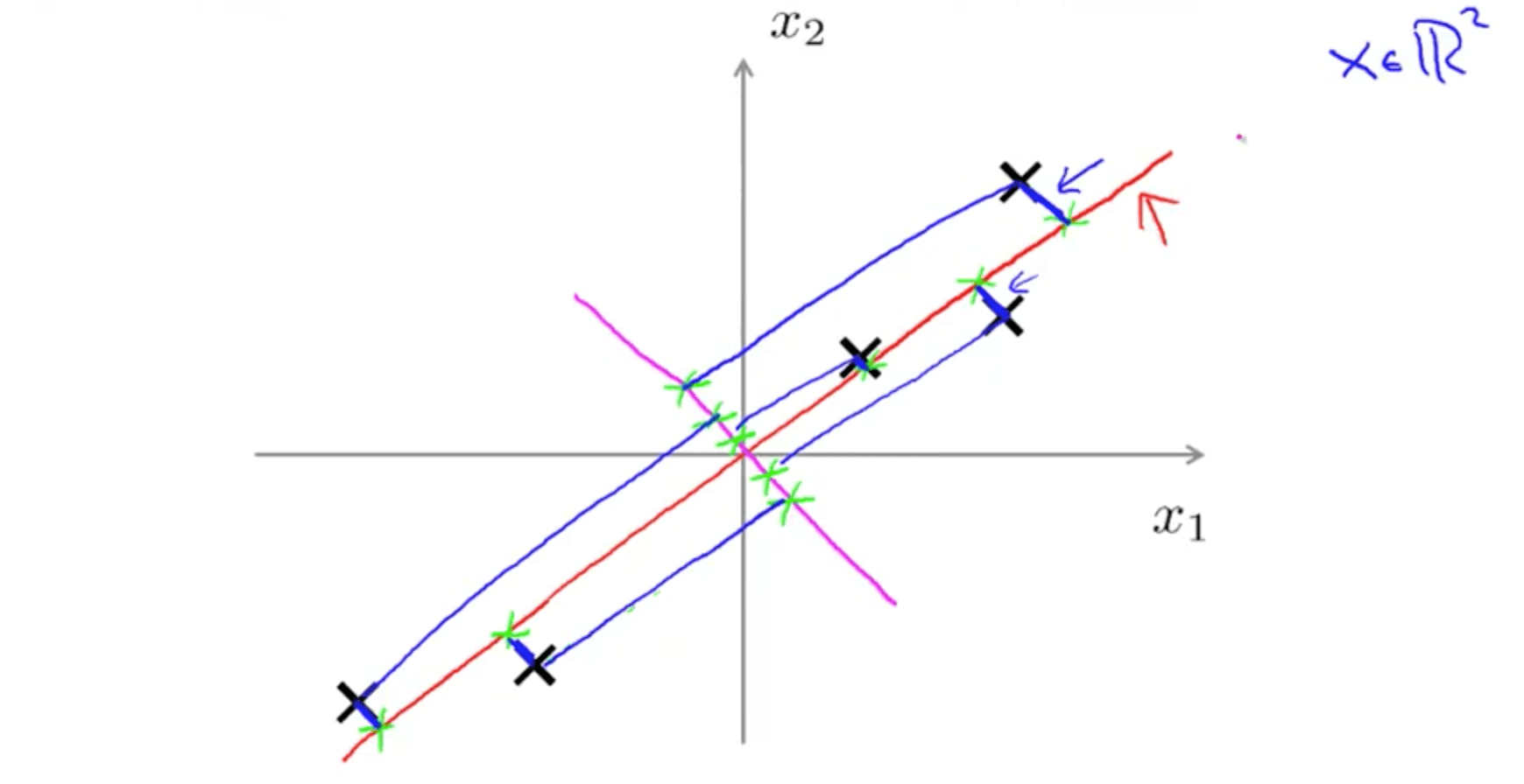
- We can project with a diagonal line (red line)
- PCA reduces the blue lines (the projection error)
- Before performing PCA, perform mean normalization (mean = 0) and feature scaling
- PCA reduces the blue lines (the projection error)
- We can also project with another diagonal line (magenta)
- But the projection errors are much larger
- Hence PCA would choose the red line instead of this magenta line
- We can project with a diagonal line (red line)
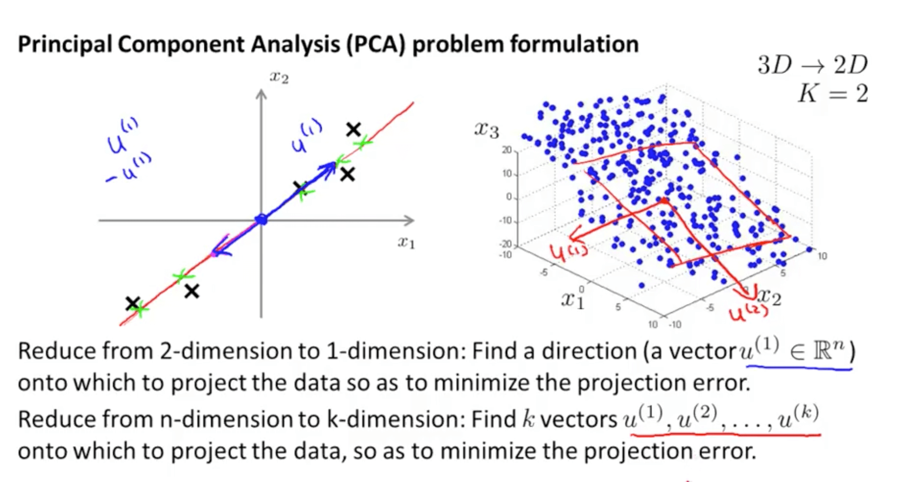
- Goal of PCA
- It’s trying to find a lower dimensional surface onto which to project the data, so as to minimize this squared projection error
- To minimize the square distance between each point and the location of where it gets projected.
- PCA is not linear regression
- PCA is a minimization of the orthogonal distance
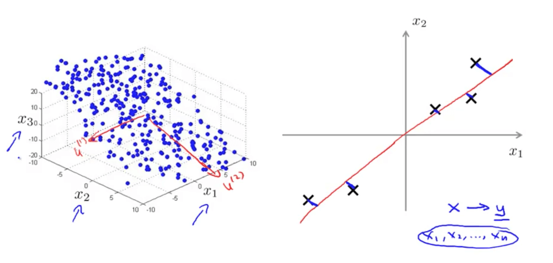
- PCA is a minimization of the orthogonal distance
2b. Principal Component Analysis Algorithm
- Data pre-processing step
- You must always do this before doing PCA
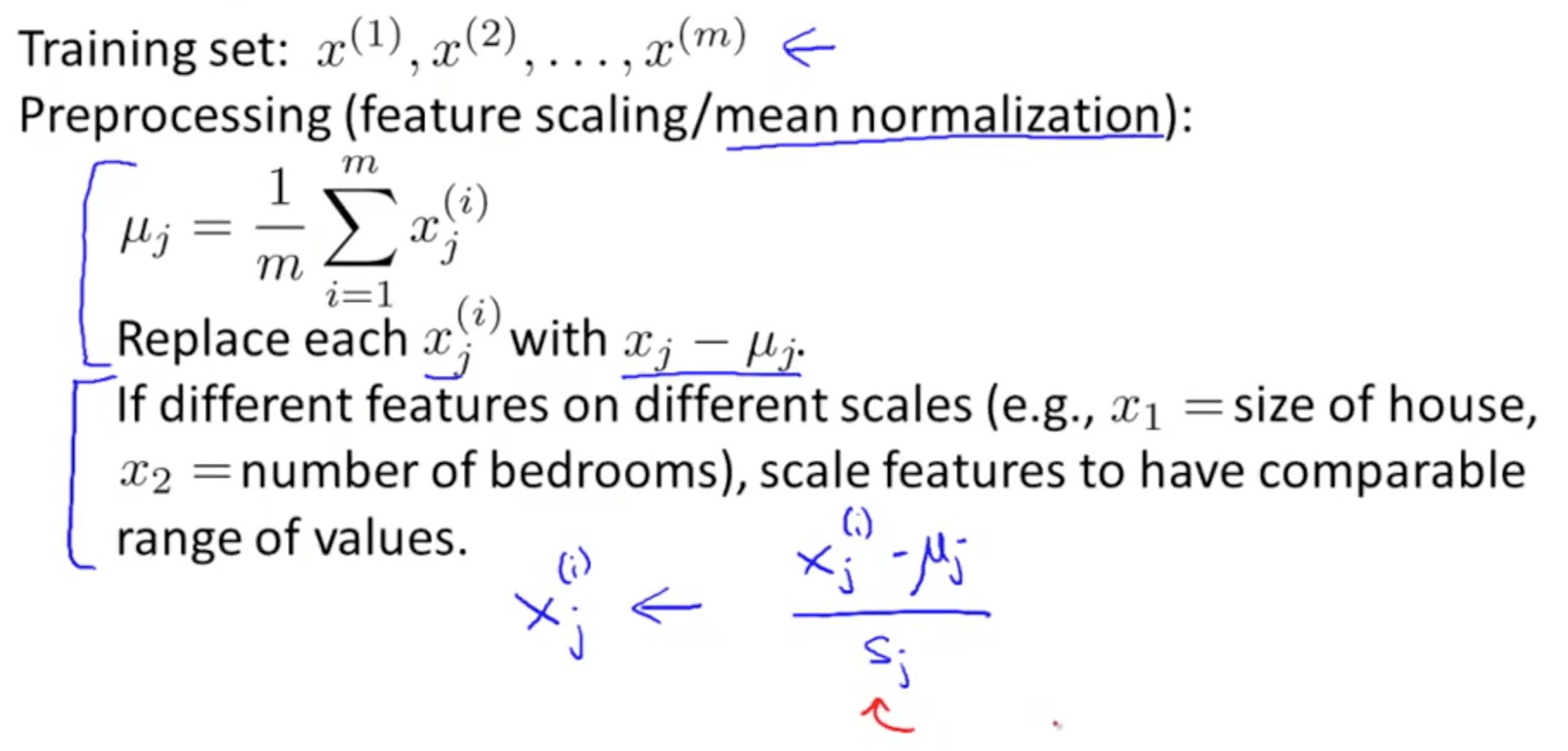
- You must always do this before doing PCA
- PCA intuition
- You need to compute the vector or vectors
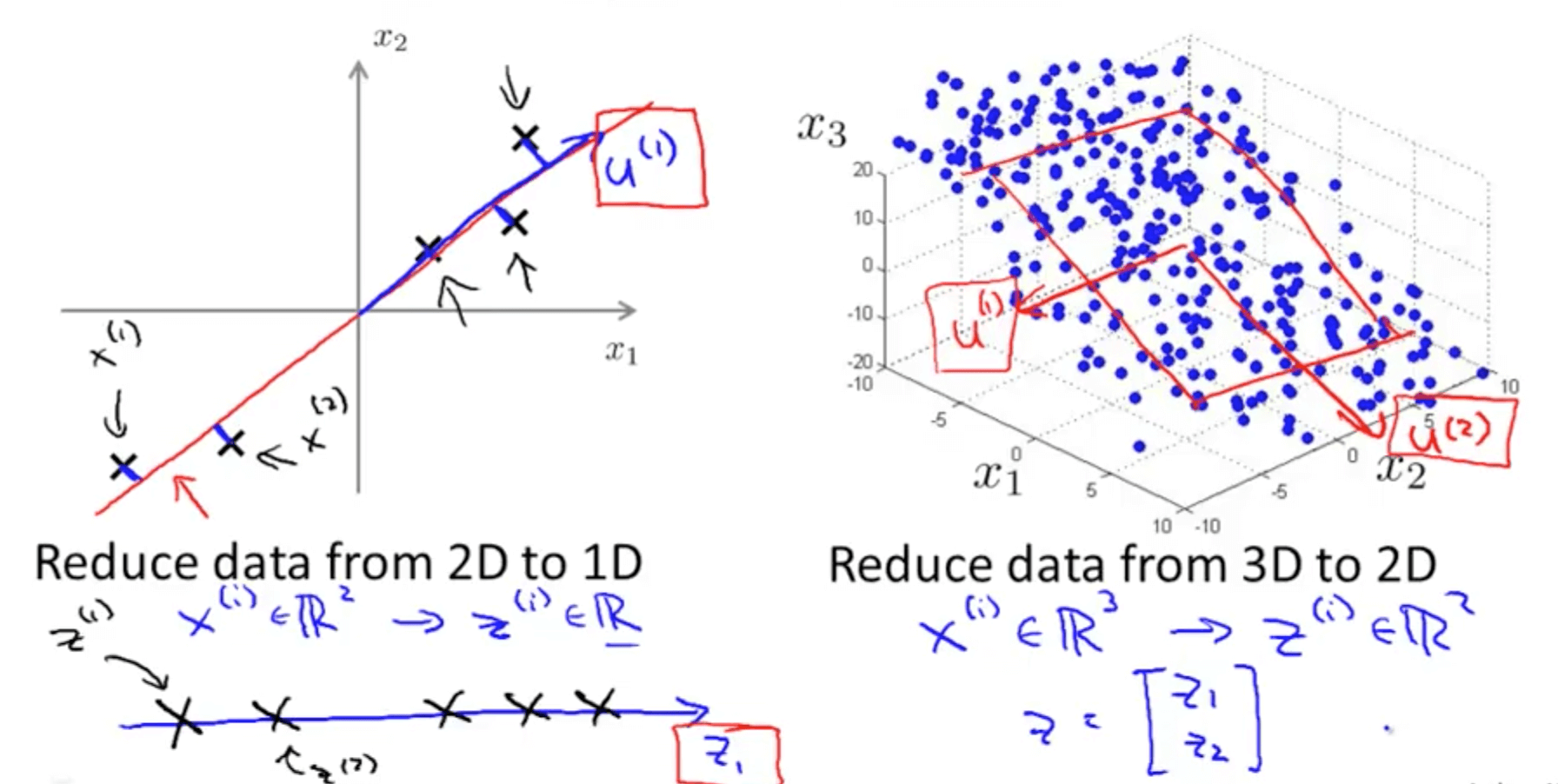
- Left graph: compute vector z(1)
- Right graph: compute vector z(1) and z(2)
- You need to compute the vector or vectors
- Procedure
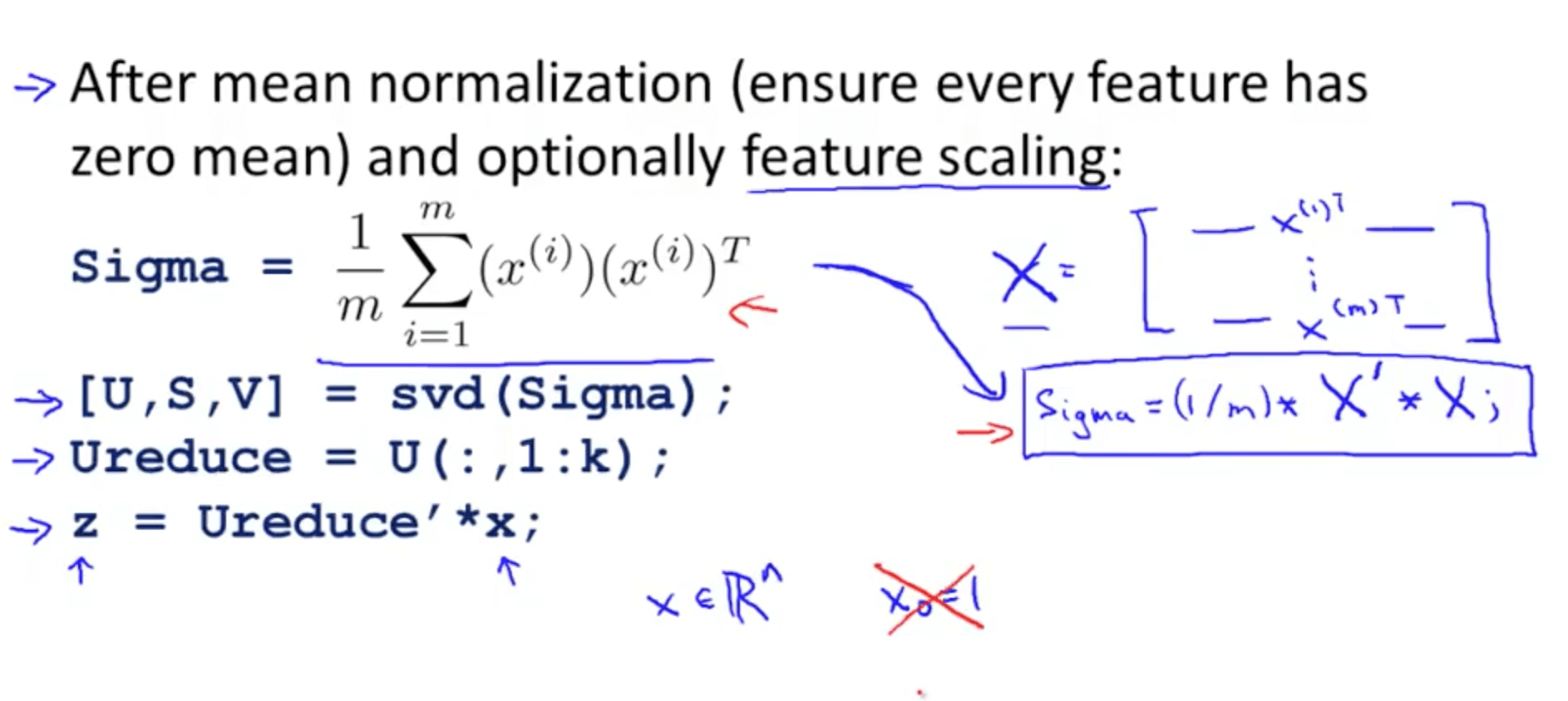
- You can use eig (eigen) or svd (singular value decomposition) but the later is more stable
- You can use any library in other languages that does singular value decomposition
- You will get 3 matrices: U, S and V
- But we only need matrix U where we manipulate to get z that is a k x 1 vector
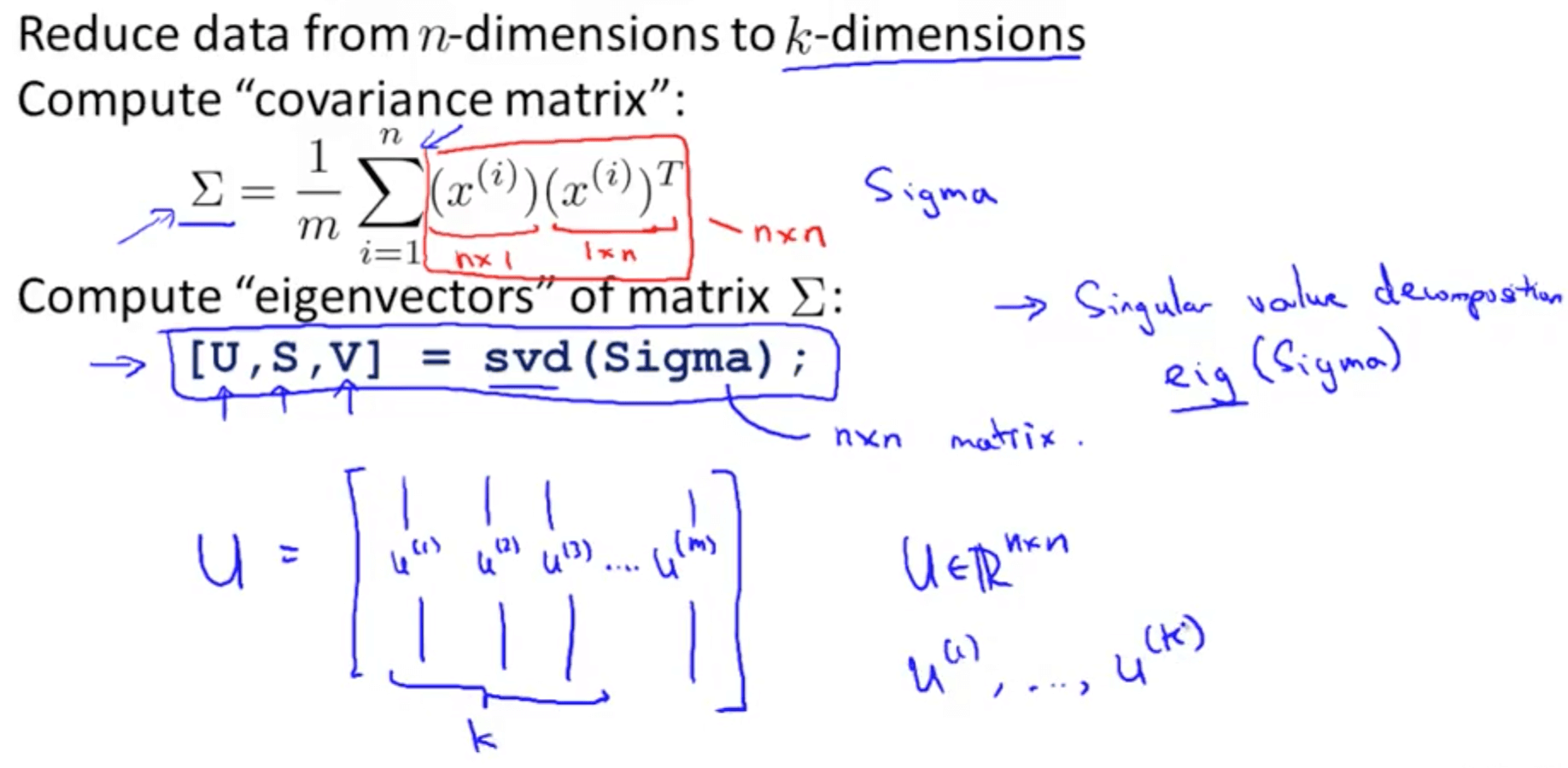
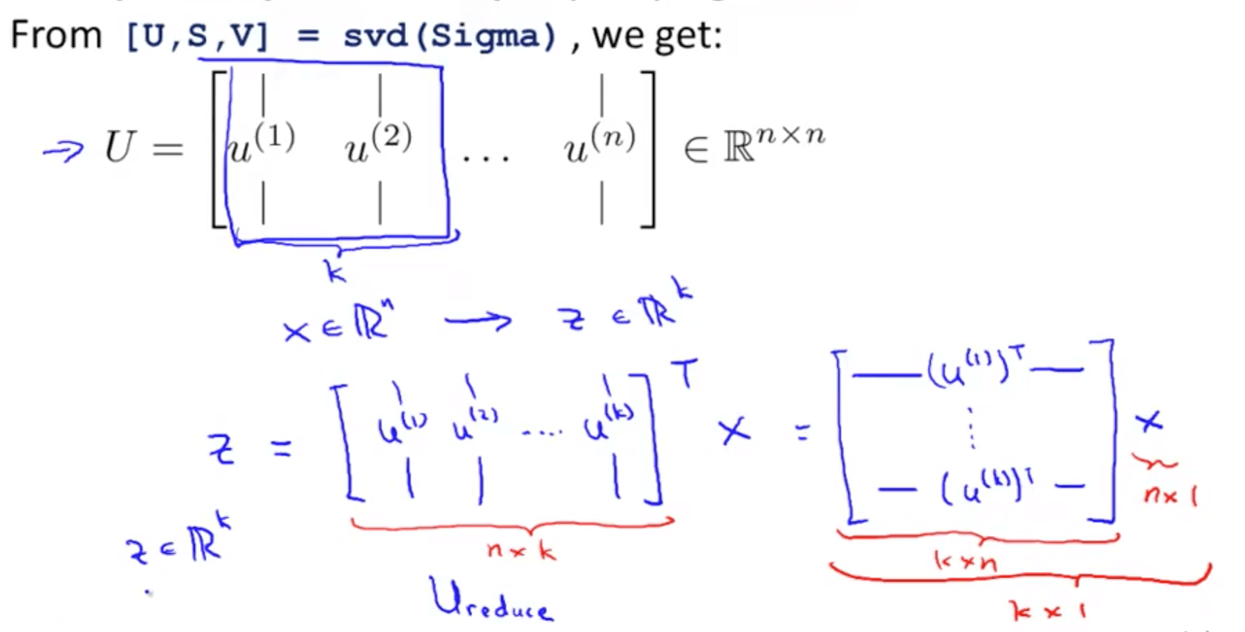
- You can use eig (eigen) or svd (singular value decomposition) but the later is more stable
- Summary of PCA algorithm in octave
3. Applying PCA
3a. Reconstruction from Compressed Representation
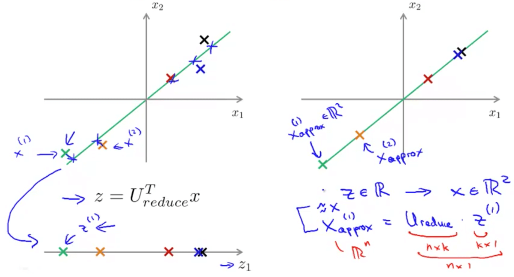
- We can go from lower dimensionality to higher dimensionality
3b. Choosing the Number of Principal Components
- k is the number of principal components
- But how do we choose k?
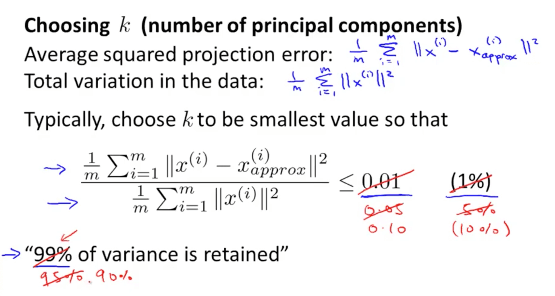
- But how do we choose k?
- There is a more efficient method on the right compared to the left
- We then use the S matrix for calculations
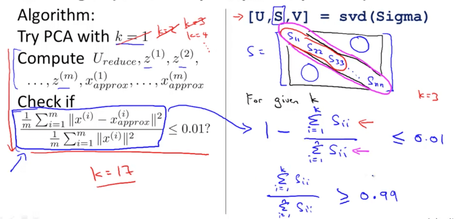
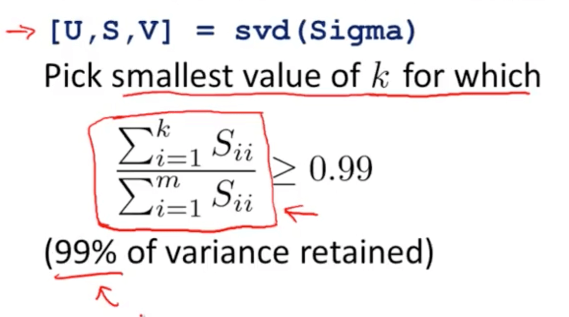
- We then use the S matrix for calculations
- You would realise that PCA can retain a high percentage of the variance even after compressing the number of dimensions of the data
3c. Advice for Applying PCA
- Supervised learning
- For many data sets, we can reduce by 5-10x easily to ensure our learning algorithm runs much faster
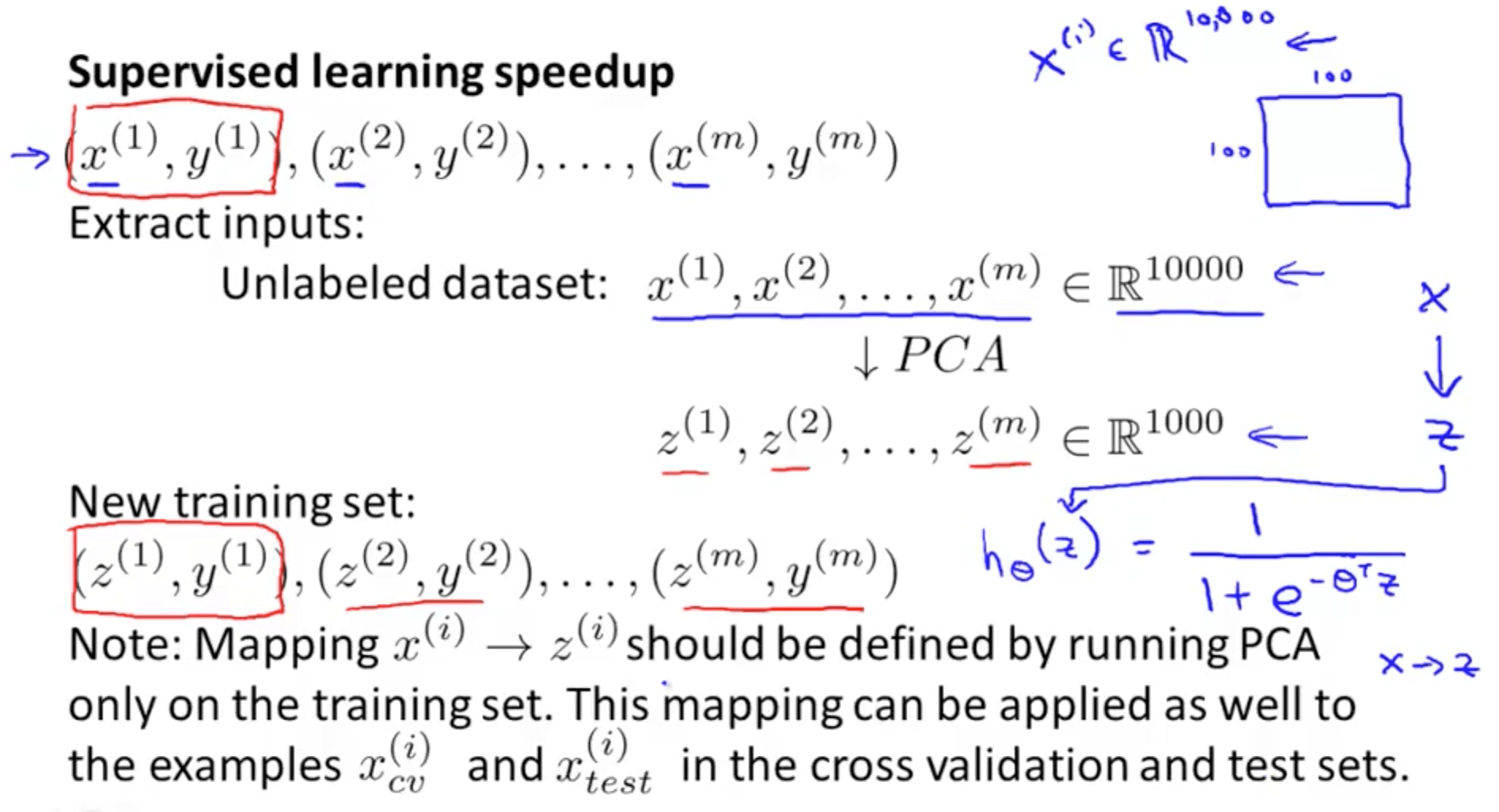
- For many data sets, we can reduce by 5-10x easily to ensure our learning algorithm runs much faster
- Application of PCA
- Compression
- Reduce memory or disk needed to store data
- Speed up learning algorithm
- We choose k by percentage of variance retained
- Visualization
- We choose only k = 2 or k = 3
- Compression
- Bad uses of PCA
- To prevent over-fitting
- Regularization is better because it is less likely to throw away valuable information as it knows the labels
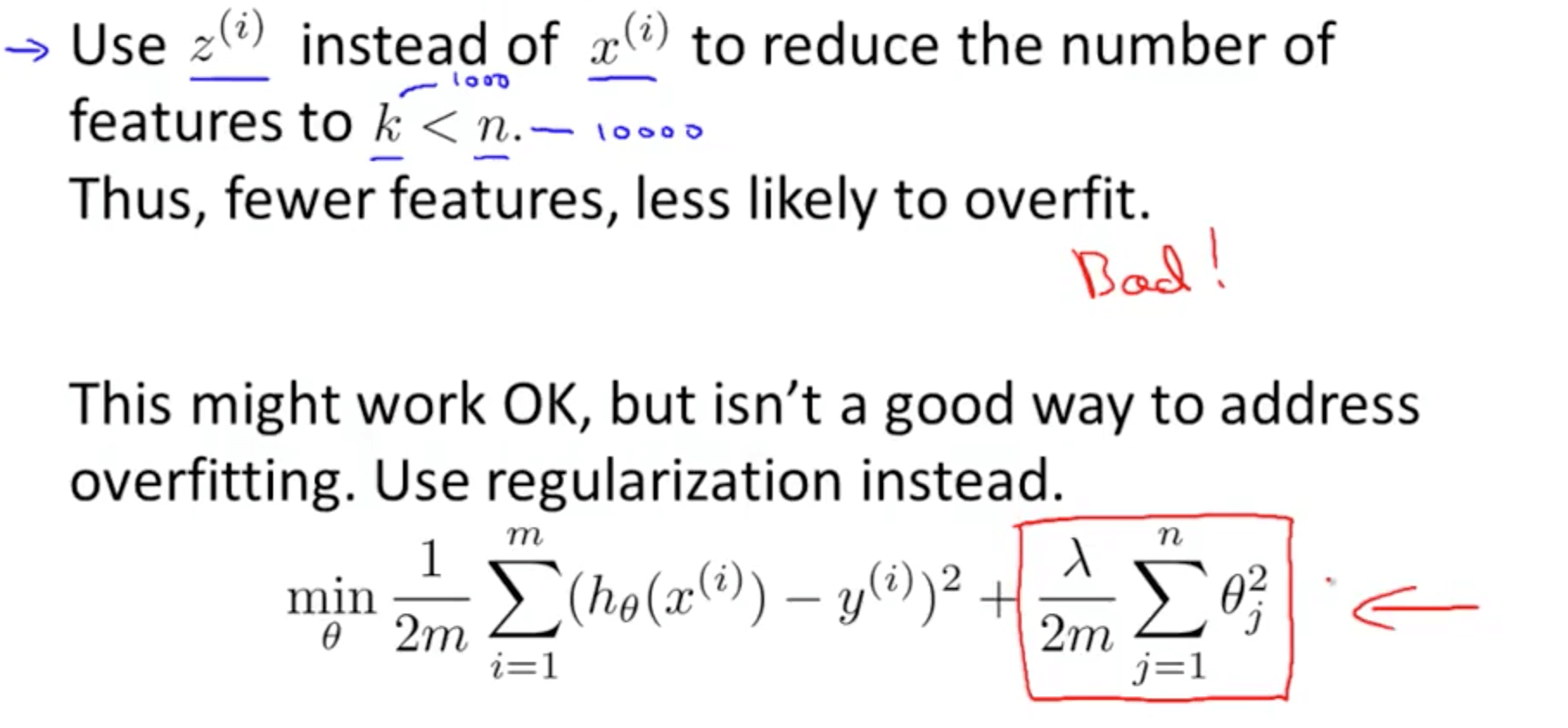
- Regularization is better because it is less likely to throw away valuable information as it knows the labels
- Running PCA without consideration
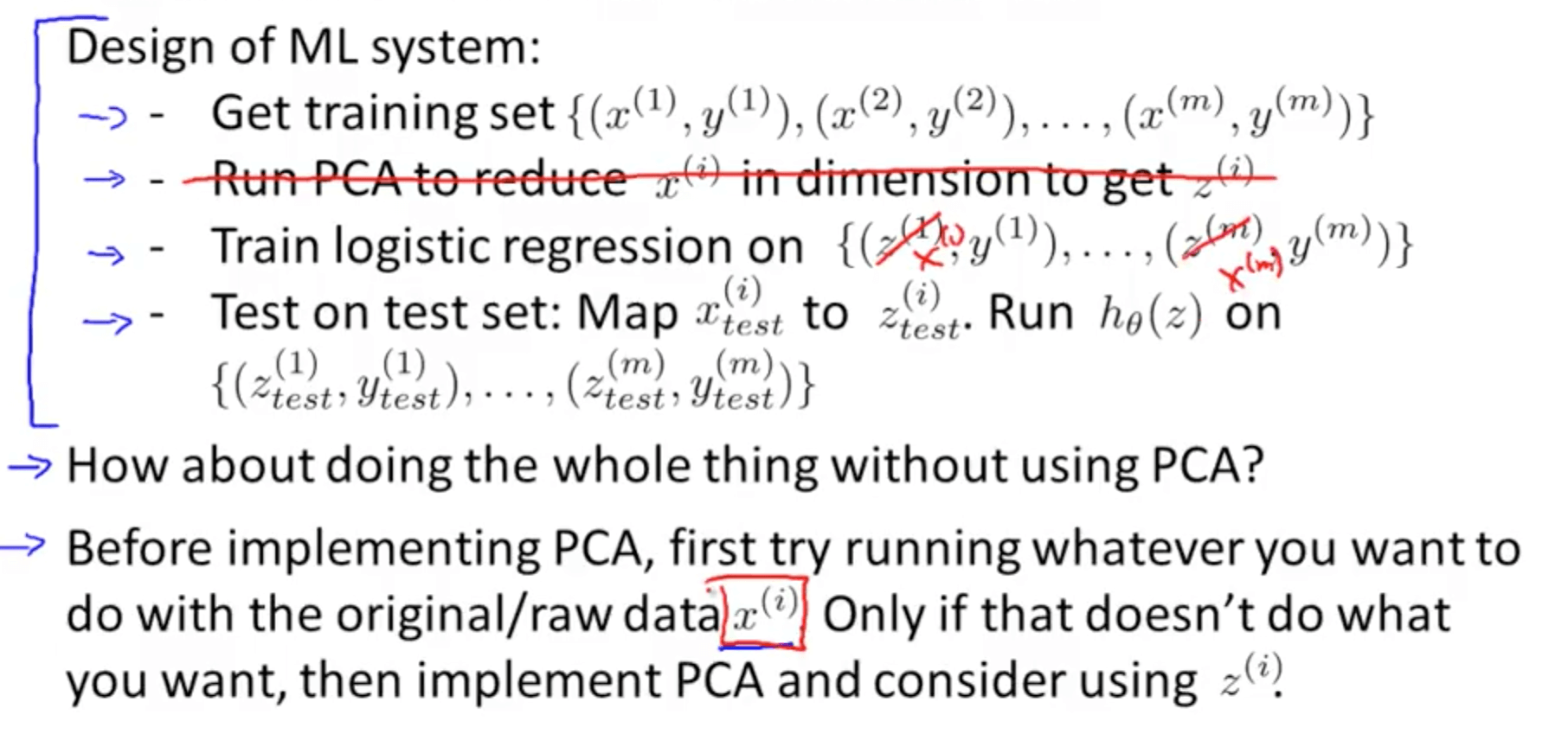
- To prevent over-fitting