Classification, logistic regression, advanced optimization, multi-class classification, overfitting, and regularization.
1. Classification and Representation
I would like to give full credits to the respective authors as these are my personal python notebooks taken from deep learning courses from Andrew Ng, Data School and Udemy :) This is a simple python notebook hosted generously through Github Pages that is on my main personal notes repository on https://github.com/ritchieng/ritchieng.github.io. They are meant for my personal review but I have open-source my repository of personal notes as a lot of people found it useful.
1a. Classification
- y variable (binary classification)
- 0: negative class
- 1: positive class
- Examples
- Email: spam / not spam
- Online transactions: fraudulent / not fraudulent
- Tumor: malignant / not malignant
- Issue 1 of Linear Regression
- As you can see on the graph, your prediction would leave out malignant tumors as the gradient becomes less steep with an additional data point on the extreme right
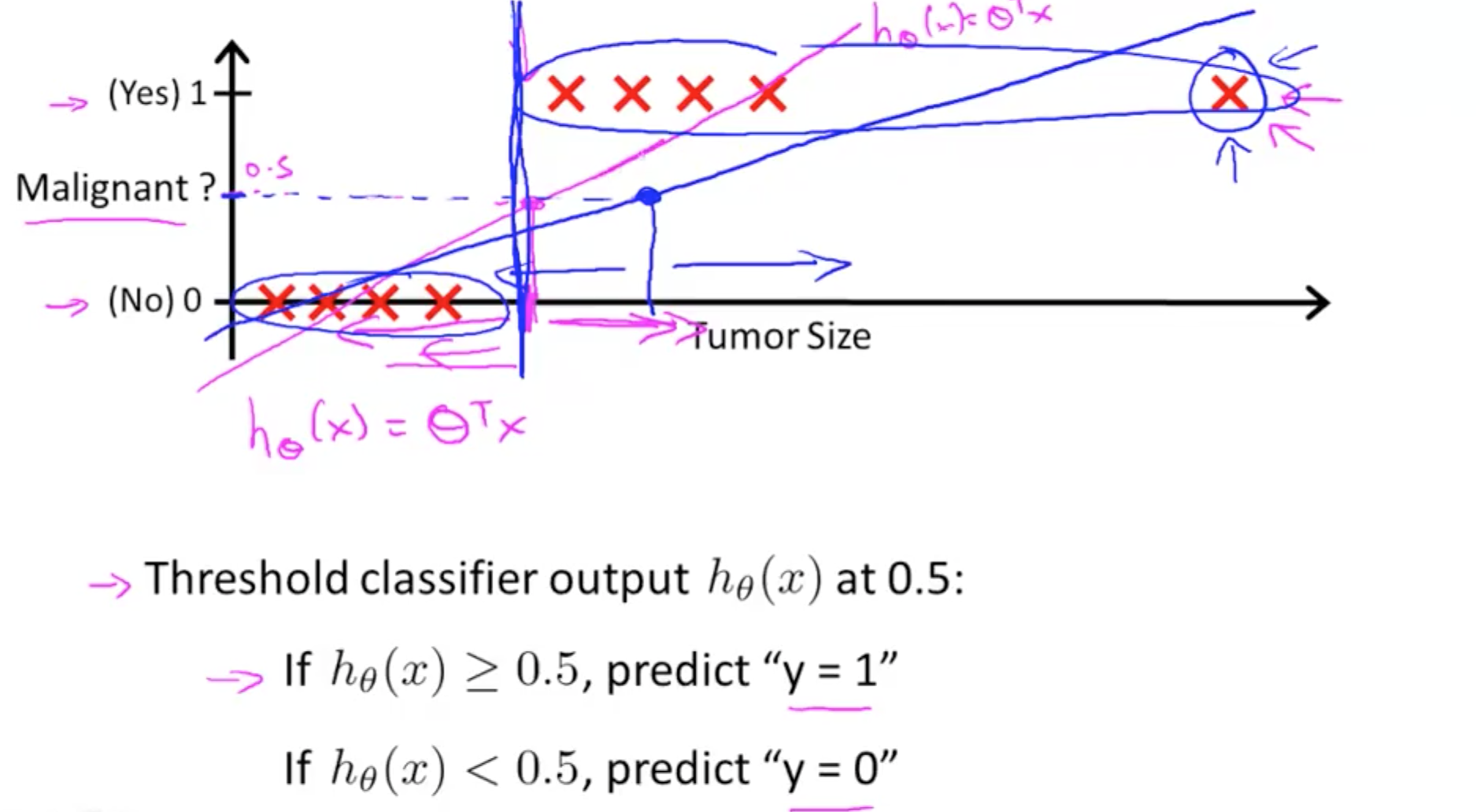
- As you can see on the graph, your prediction would leave out malignant tumors as the gradient becomes less steep with an additional data point on the extreme right
- Issue 2 of Linear Regression
- Hypothesis can be larger than 1 or smaller than zero
- Hence, we have to use logistic regression
1b. Logistic Regression Hypothesis
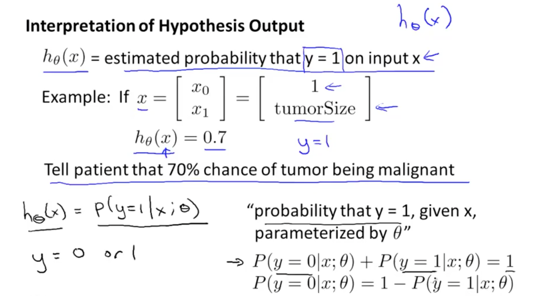
- Logistic Regression Model
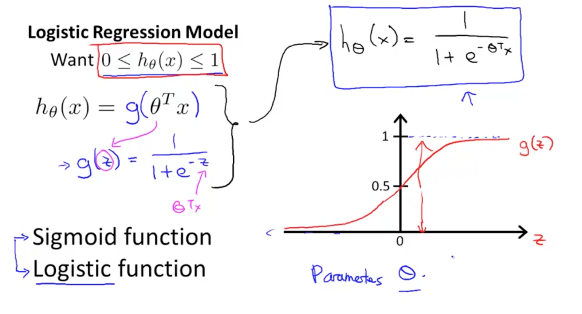
- Interpretation of Hypothesis Output
1c. Decision Boundary
- Boundaries
- Max 1
- Min 0
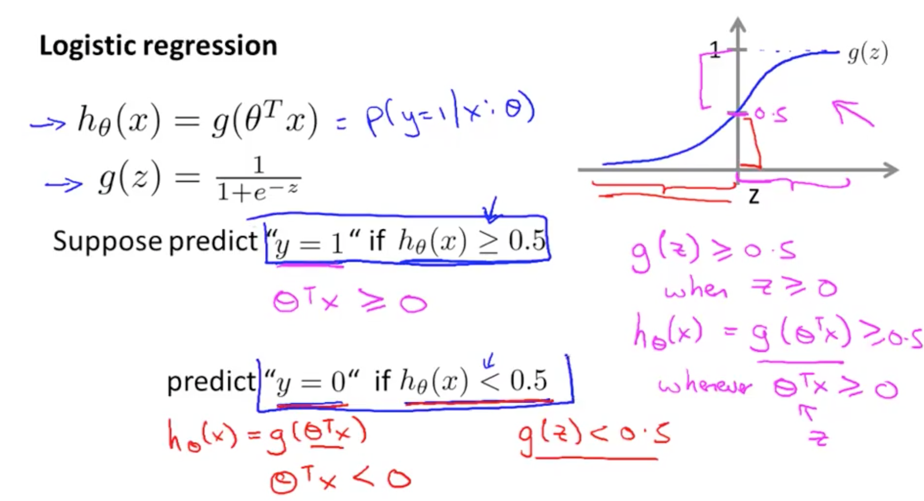
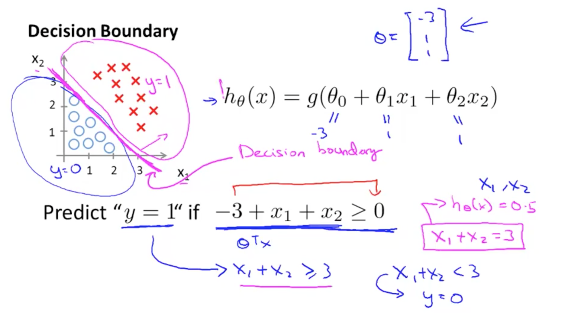
- Boundaries are properties of the hypothesis not the data set
- You do not need to plot the data set to get the boundaries
- This will be discussed subsequently
- Non-linear decision boundaries
- Add higher order polynomial terms as features
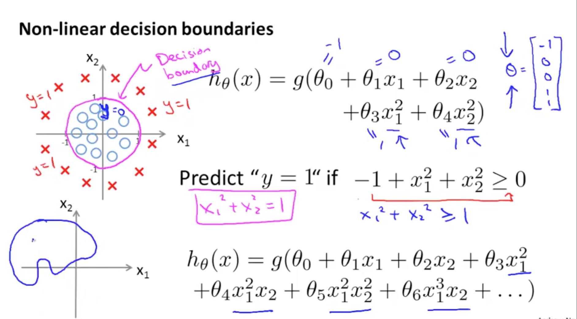
- Add higher order polynomial terms as features
2. Logistic Regression Model
2a. Cost Function
- How do we choose parameters?
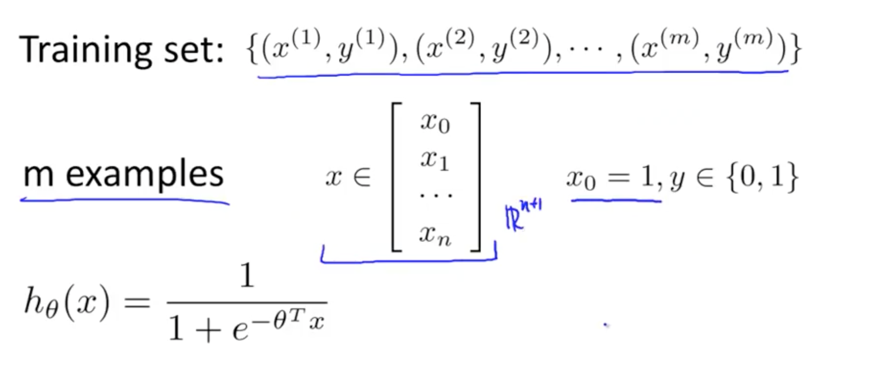
- If y = 1
- If h(x) = 0 & y = 1, costs infinite
- If h(x) = 1 & y = 1
, costs = 0

- If y = 0
- If h(x) = 0 & y = 0, costs = 0
- If h(x) = 1 & y = 0, costs infinite

2b. Simplified Cost Function & Gradient Descent
- Simplified Cost Function Derivatation
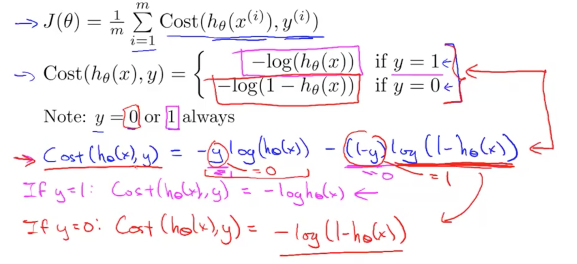
- Simplified Cost Function
- Always convex so we will reach global minimum all the time
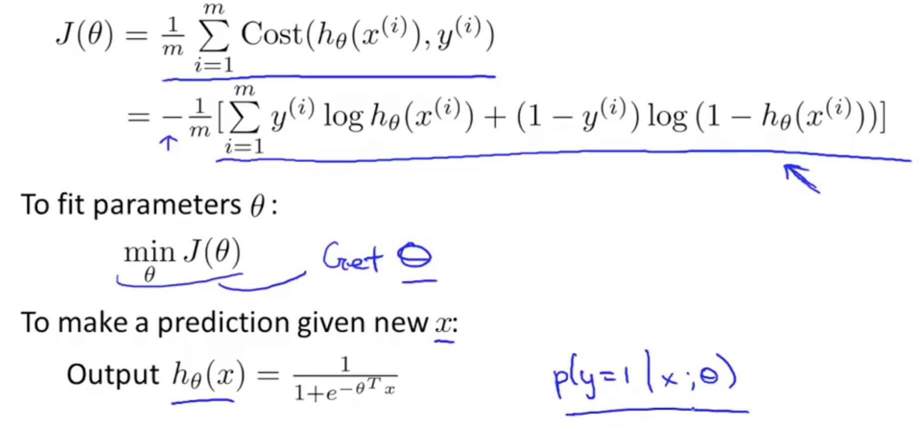
- Always convex so we will reach global minimum all the time
- Gradient Descent
- It looks identical, but the hypothesis for Logistic Regression is different from Linear Regression
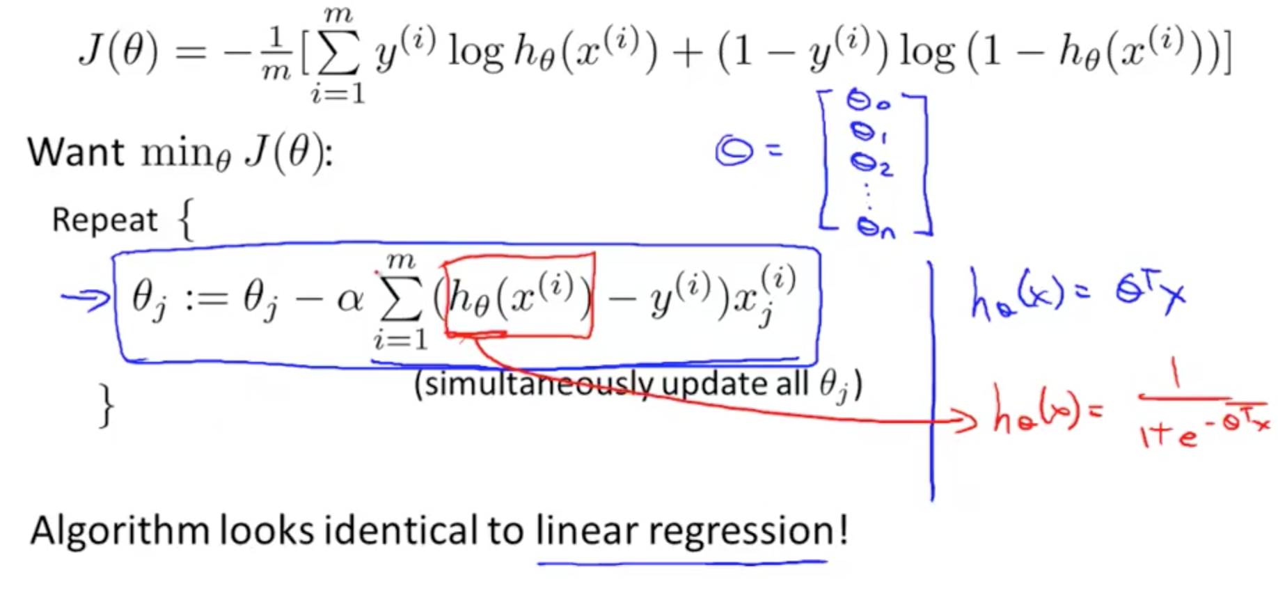
- It looks identical, but the hypothesis for Logistic Regression is different from Linear Regression
- Ensuring Gradient Descent is Running Correctly

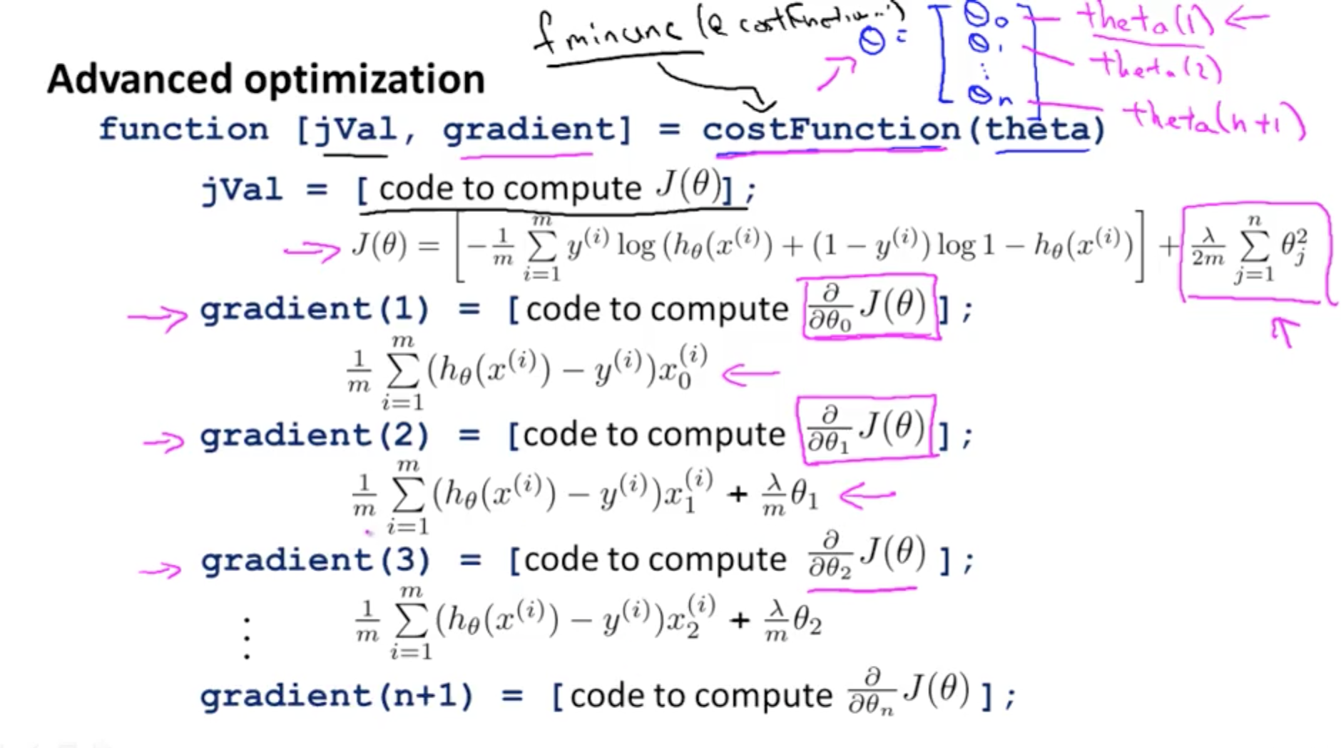
2c. Advanced Optimization
- Background
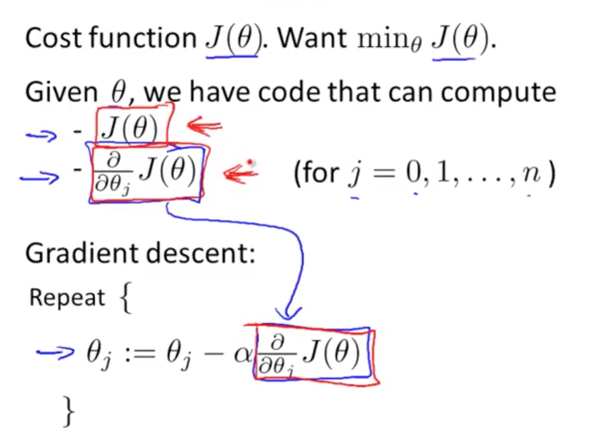
- Optimization algorithm
- Gradient descent
- Others
- Conjugate gradient
- BFGS
- L-BFGS
- Advantages “Others”
- No need to manually pick alpha
- Often faster than gradient descent
- Disadvantages “Others”
- More complex
- Should not implement these yourself unless you’re an expert in numerical computing
- Use a software library to do them
- There are good and bad implementations, choose wisely
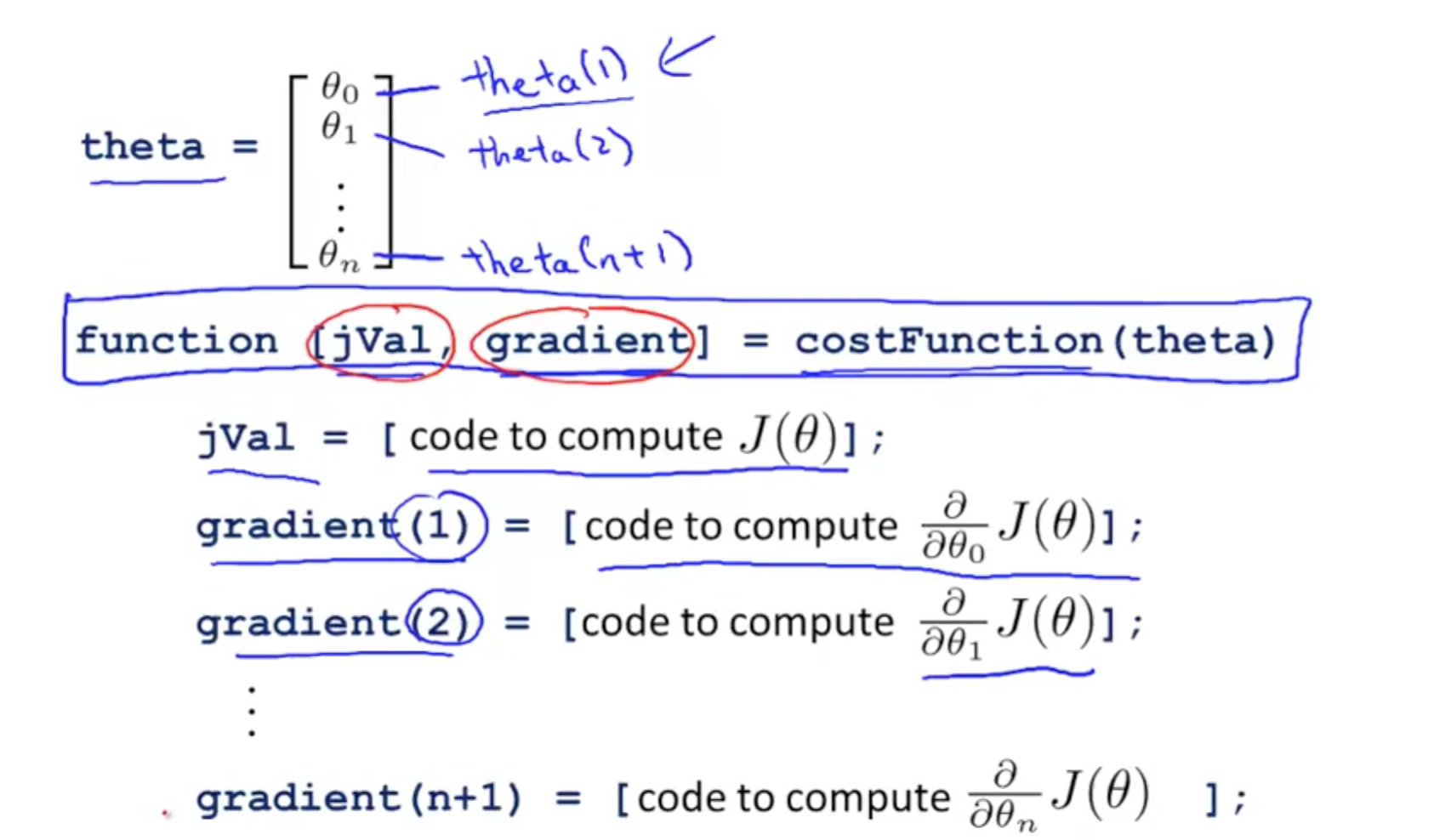
- Components of code explanation
- Code
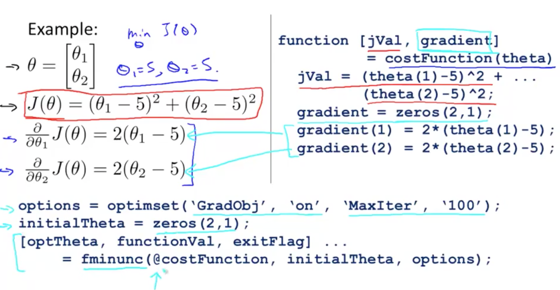
- ‘Gradobj’, ‘on’
- We will be providing gradient to this algorithm
- ‘MaxIter’, ‘100’
- Max iterations to 100
- fminunc
- Function minimisation unconstrained
- Cost minimisation function in octave
- @costFunction
- Points to our defined function
- optTheta
- Automatically choose learning rate
- Gradient descent on steriods
- Results
- Theta0 = 5
- Theta1 = 5
- functionVal = 1.5777e-030
- Essentially 0 for J(theta), what we are hoping for
- exitFlag = 1
- Verify if it has converged, 1 = converged
- Theta must be more than 2 dimensions
- Main point is to write a function that returns J(theta) and gradient to apply to logistic or linear regression
- Code
3. Multi-class Classification
- Similar terms
- One-vs-all
- One-vs-rest
- Examples
- Email folders or tags (4 classes)
- Work
- Friends
- Family
- Hobby
- Medical Diagnosis (3 classes)
- Not ill
- Cold
- Flu
- Weather (4 classes)
- Sunny
- Cloudy
- Rainy
- Snow
- Email folders or tags (4 classes)
- Binary vs Multi-class
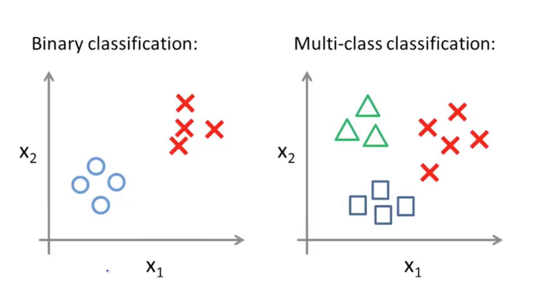
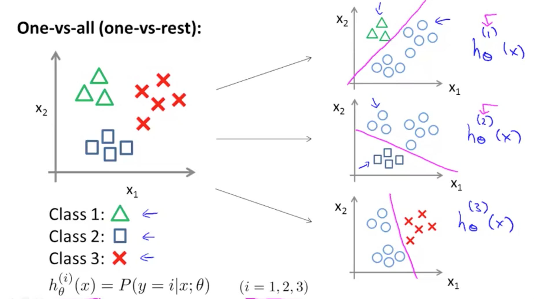
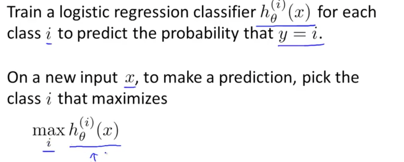
- One-vs-all (One-vs-rest)
- Split them into 3 distinct groups and compare them to the rest
- If you have k classes, you need to train k logistic regression classifiers
4. Solving Problem of Overfitting
4a. Problem of Overfitting
- Linear Regression: Overfitting
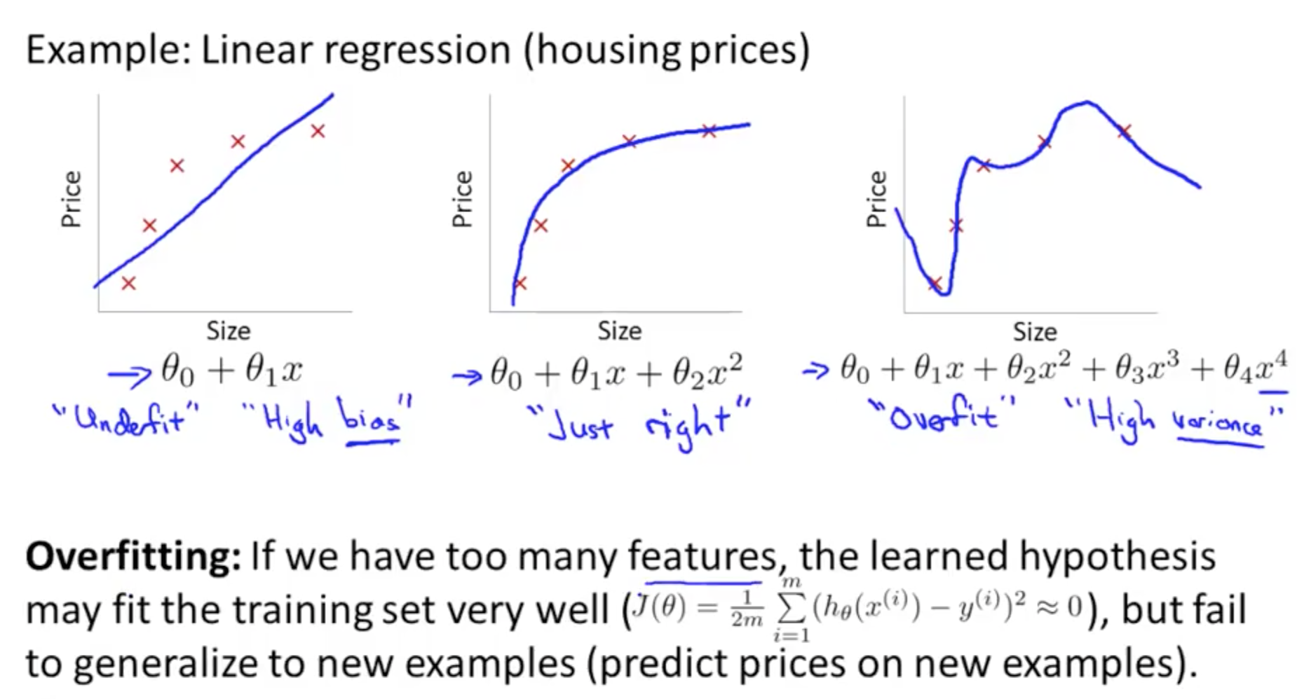
- Overfit
- High Variance
- Too many features
- Fit well but fail to generalize new examples
- Underfit
- High Bias
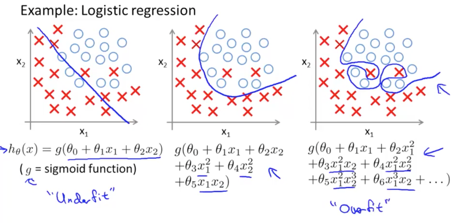
- Overfit
- Logistic Regression: Overfitting
- Solutions to Overfitting
- Reduce number of features
- Manually select features to keep
- Model selection algorithm
- Regularization
- Keep all features, but reduce magnitude or values of parameters theta_j
- Works well when we’ve a lot of features
- Reduce number of features
4b. Cost Function
- Intuition
- Making theta so small that is almost equivalent to zero
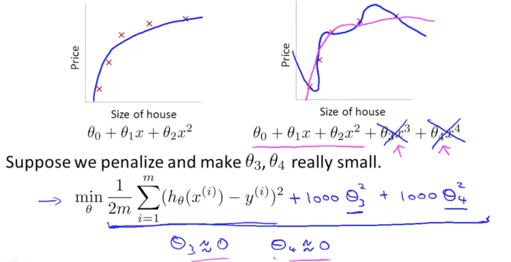
- Making theta so small that is almost equivalent to zero
- Regularization
- Small values for parameters (thetas)
- “Simpler” hypothesis
- Less prone to overfitting
- Add regularization parameter to J(theta) to shrink parameters
- First goal: fit training set well (first term)
- Second goal: keep parameter small (second, pink, term)
- If lamda is set to an extremely large value, this would result in underfitting
- High bias
- Only penalize thetas from 1, not from 0
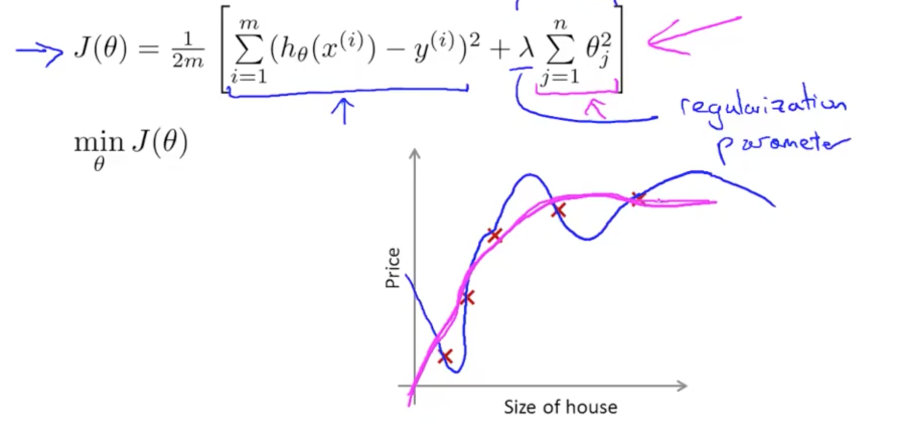
- Small values for parameters (thetas)
4c. Regularized Linear Regression
- Gradient Descent Equation
- Usually, (1- alpha * lambda / m) is 0.99
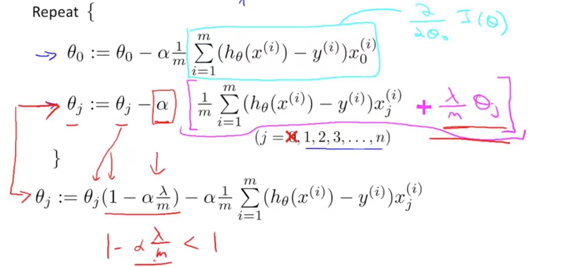
- Usually, (1- alpha * lambda / m) is 0.99
- Normal Equation
- Alternative to minimise J(theta) only for linear regression
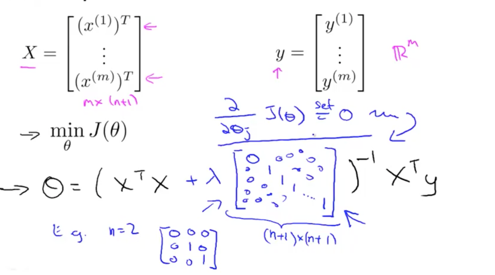
- Alternative to minimise J(theta) only for linear regression
- Non-invertibility
- Regularization takes care of non-invertibility
- Matrix will not be singular, it will be invertible
4c. Regularized Logistic Regression
- Cost function with regularization
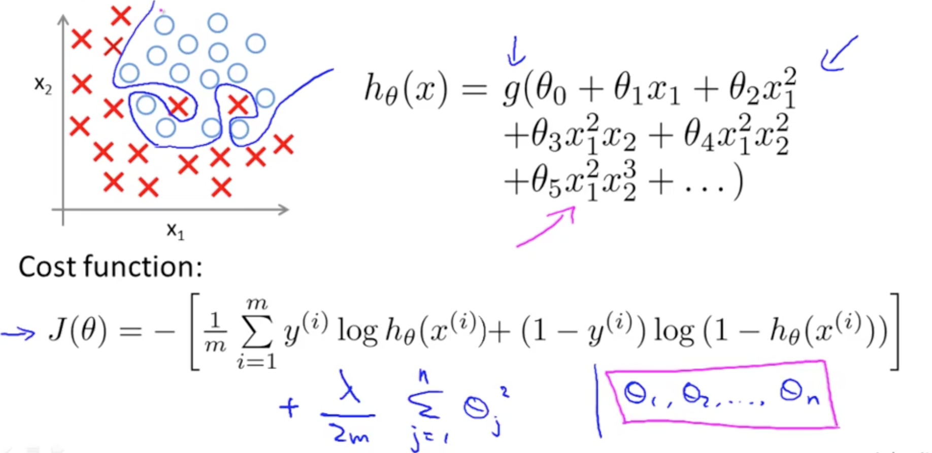
- Using Gradient Descent for Regularized Logistic Regression Cost Function
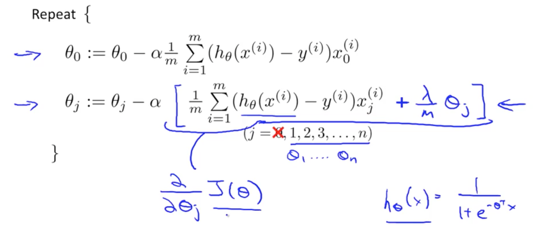
- To check if Gradient Descent is working well

- Using Advanced Optimisation
- Pass in fminunc in costFunction
- costFunction need to return
- jVal
- gradient
